React Hard: The First Law Gets Chemical
![]()
Introduction
React Hard: The First Law Gets Chemical and
React Harder: Formation Heats and Alternate Endings
present
- three sets of calculations for the 1st Law in reacting systems.
- based on A Combustible Mixture! video
- Review A Combustible Mixture! before watching these two.
Sample Combustion Calculations
\(2.00\ \mathrm{kmol/s}\) of propane at \(20\ ^\circ\mathrm{C}\) are burned in 25% excess dry air \(30\ ^\circ\mathrm{C}\) in a faulty combustor. 100% of the hydrogen combusts to form water, but only 80% of the carbon combusts completely to \(\mathrm{CO_2}\). The remainder combusts to \(\mathrm{CO}\).
- Calculate the molar flow rates of the reactants and products.
- Calculate the adiabatic flame temperature.
- Calculate the mass flow rate of saturated steam at \(100\ ^\circ\mathrm{C}\) that can be produced from entering water at \(25\ ^\circ\mathrm{C}\) if the exhaust exits at \(300\ ^\circ\mathrm{C}\) below the adiabatically flame temperature.
Solution
First, the summary of the mole balance on the process. There are multiple sets of chemical equations we could write. We will consider two sets:
First Set \[
\mathrm{C_3H_8 + 5O_2} \rightarrow \mathrm{3CO_2 + 4 H_2O}
\tag{1}\]
\[
\mathrm{C_3H_8 + \frac{7}{2}O_2} \rightarrow \mathrm{3CO + 4H_2O}
\tag{2}\]
Second Set: \[
\mathrm{C_3H_8 + \frac{7}{2}O_2} \rightarrow \mathrm{3CO + 4H_2O}
\tag{3}\]
\[
\mathrm{CO + \frac{1}{2}O_2} \rightarrow \mathrm{CO_2}
\tag{4}\]
Solution (cont.)
For calculating excess, complete combustion is calculated with Equation 1.
\[
\dot{n}_\mathrm{O_2stoic} = \frac{\nu_\mathrm{O_2}}{\nu_\mathrm{C_3H_8}} \dot{n}_\mathrm{C_3H_8stoic} = \frac{-5}{-1}(2\ \mathrm{kmol/s}) = 10\ \mathrm{kmol/s}
\]
\[
\mathrm{frac.\ xs} = 0.25 = \frac{ \dot{n}_\mathrm{O_2in} - \dot{n}_\mathrm{O_2stoic} }{\dot{n}_\mathrm{O_2stoic}}
\]
\[
\dot{n}_\mathrm{O_2in} = (1 + \mathrm{frac.\ xs})\dot{n}_\mathrm{O_2stoic} = 1.25(10\ \mathrm{kmol/s})= 12.5\ \mathrm{kmol/s}
\]
\[
\dot{n}_\mathrm{N_2in} = \frac{79}{21}\dot{n}_\mathrm{O_2in} = \frac{79}{21}(12.5\ \mathrm{kmol/s}) = 47.0\ \mathrm{kmol/s}
\]
\[
\dot{n}_\text{Air-in} = \dot{n}_\mathrm{O_2in} + \dot{n}_\mathrm{N_2in} = 12.5 + 47.0 = \boxed{ 59.5\ \mathrm{kmol/s}}
\]
Solution (cont.)
The full set of mole balances with Equation 1 and Equation 2 is
\[
\dot{n}_\mathrm{C_3H_8out} = \dot{n}_\mathrm{C_3H_8in} - \dot{\xi}_1 - \dot{\xi}_2 \implies \dot{\xi}_1 + \dot{\xi}_2 = 2\ \mathrm{kmol/s}
\]
\[
\dot{n}_\mathrm{CO_2out} = \dot{n}_\mathrm{CO_2in} + 3\dot{\xi}_1 + 0 \boldsymbol{\cdot} \dot{\xi}_2 \implies \dot{n}_\mathrm{CO_2out} = 3\dot{\xi}_1
\]
\[
\dot{n}_\mathrm{COout} = \dot{n}_\mathrm{COin} + 0 \boldsymbol{\cdot} \dot{\xi}_1 + 3 \dot{\xi}_2 \implies \dot{n}_\mathrm{COout} = 3\dot{\xi}_2
\]
\[
\dot{n}_\mathrm{O_2out} = \dot{n}_\mathrm{O_2in} - 5\dot{\xi}_1 - 3.5 \dot{\xi}_2 = 12.50\ \mathrm{kmol/s} - 5\dot{\xi}_1 - 3.5 \dot{\xi}_2
\]
\[
\dot{n}_\mathrm{N_2out} = \dot{n}_\mathrm{N_2in} + 0 \boldsymbol{\cdot} \dot{\xi}_1 +0 \boldsymbol{\cdot} \dot{\xi}_2 = \boxed{ 47.0\ \mathrm{kmol/s} }
\]
\[
\dot{n}_\mathrm{H_2Oout} = \dot{n}_\mathrm{H_2Oin} + 4 \dot{\xi}_1 + 4 \dot{\xi}_2 = 4 \dot{\xi}_1 + 4 \dot{\xi}_2
\]
Solution (cont.)
Applying the \(\mathrm{CO_2}\)-to-\(\mathrm{CO}\) constraint
\[
\frac{\dot{n}_\mathrm{COout}}{\dot{n}_\mathrm{CO_2out}} = \frac{1 - 0.80}{0.80}=0.25 = \frac{3\dot{\xi}_2}{3\dot{\xi}_1} = \frac{\dot{\xi}_2}{\dot{\xi}_1}
\]
\[
\dot{\xi}_1 + \dot{\xi}_2 = 2\ \mathrm{kmol/s} = \dot{\xi}_1 + 0.25 \dot{\xi}_1 = 1.25 \dot{\xi}_1
\]
\[
\implies \dot{\xi}_1 = 1.6\ \mathrm{kmol/s},\ \dot{\xi}_2 = 0.4\ \mathrm{kmol/s}
\]
\[
\dot{n}_\mathrm{O_2out} = 12.5\ \mathrm{kmol/s} - 5 \boldsymbol{\cdot} 1.6 - 3.5 \boldsymbol{\cdot} 0.4 = \boxed{ 3.10\ \mathrm{kmol/s} }
\]
\[
\dot{n}_\mathrm{H_2Oout} = 4 \boldsymbol{\cdot} 1.6 + 4 \boldsymbol{\cdot} 0.4 = \boxed{ 8.00\ \mathrm{kmol/s} }
\]
\[
\implies \dot{n}_\mathrm{CO_2out} = 3 \boldsymbol{\cdot} 1.6\ \mathrm{kmol/s} = \boxed{ 4.8\ \mathrm{kmol/s} },
\]
\[
\dot{n}_\mathrm{COout} = 3 \boldsymbol{\cdot} 0.4\ \mathrm{kmol/s} = \boxed{ 1.2\ \mathrm{kmol/s} }
\]
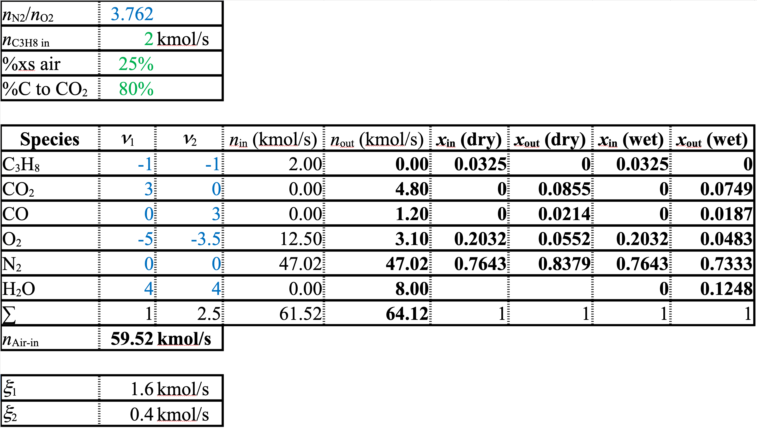
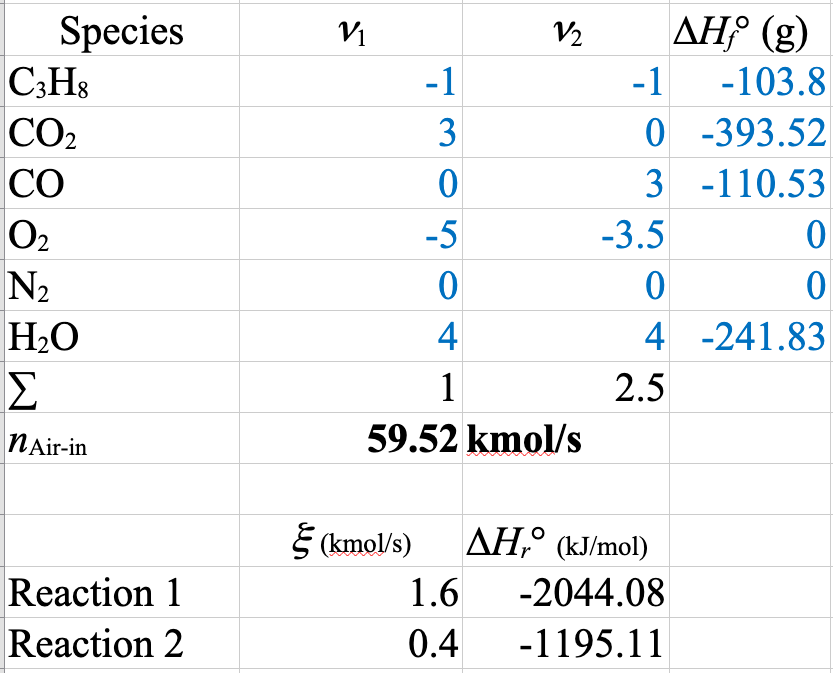
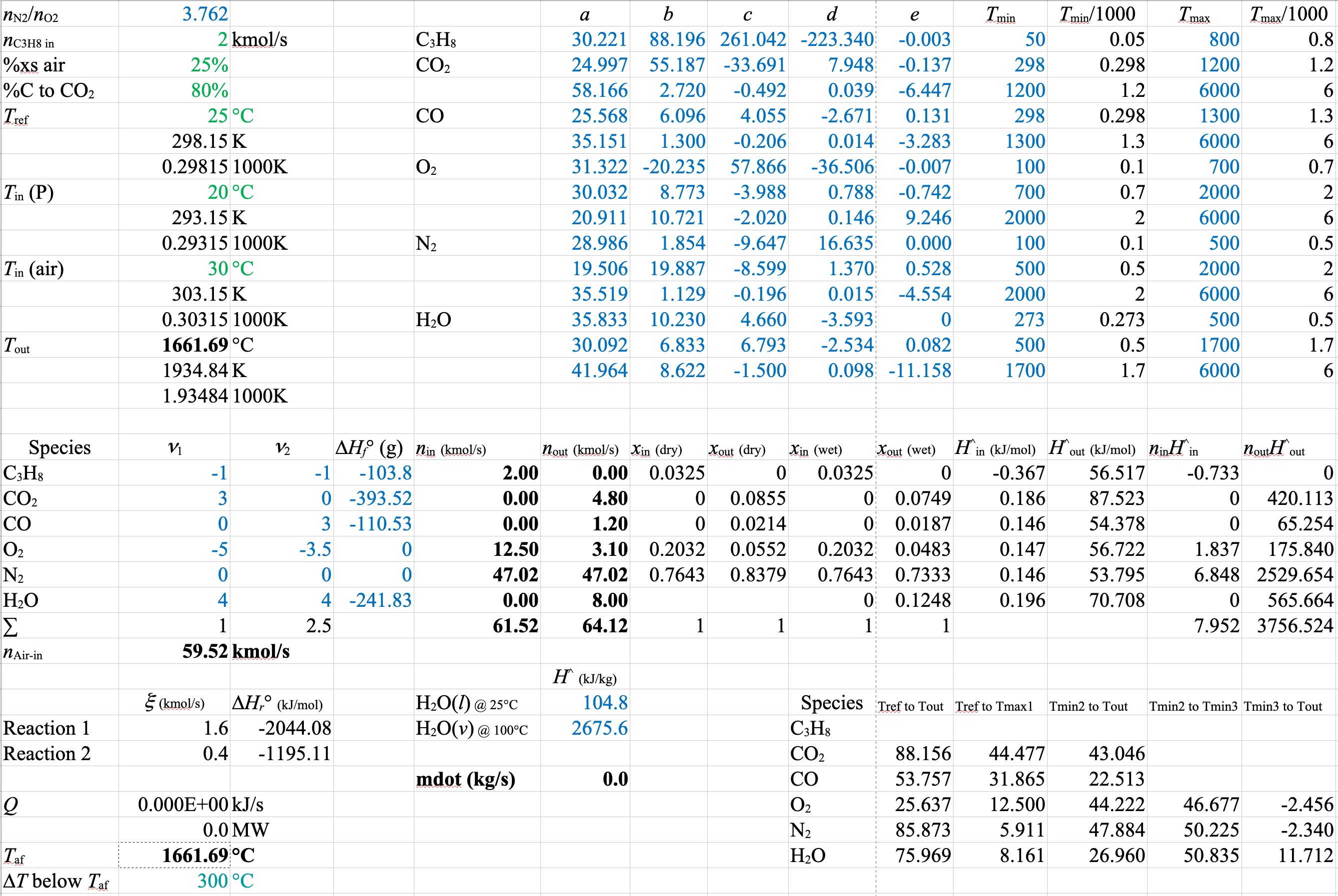
Solution (cont.)
A spreadsheet of the solution is shown below
![]()
Solution (cont.)
The full set of mole balances with Equation 3 and Equation 4 is
\[
\dot{n}_\mathrm{C_3H_8out} = \dot{n}_\mathrm{C_3H_8in} - \dot{\xi}_3 \implies \dot{\xi}_3 = 2\ \mathrm{kmol/s}
\]
\[
\dot{n}_\mathrm{CO_2out} = \dot{n}_\mathrm{CO_2in} + \dot{\xi}_4 \implies \dot{n}_\mathrm{CO_2out} = \dot{\xi}_4
\]
\[
\dot{n}_\mathrm{COout} = \dot{n}_\mathrm{COin} + 3 \dot{\xi}_3 - \dot{\xi}_4 \implies \dot{n}_\mathrm{COout} = 6\ \mathrm{kmol/s} - \dot{\xi}_4
\]
\[
\dot{n}_\mathrm{O_2out} = \dot{n}_\mathrm{O_2in} - 3.5 \dot{\xi}_3 - 0.5 \dot{\xi}_4 = 12.50\ \mathrm{kmol/s} - 7\ \mathrm{kmol/s} - 0.5 \dot{\xi}_4
\]
\[
\dot{n}_\mathrm{N_2out} = \dot{n}_\mathrm{N_2in} = 47.0\ \mathrm{kmol/s}
\]
\[
\dot{n}_\mathrm{H_2Oout} = \dot{n}_\mathrm{H_2Oin} + 4 \dot{\xi}_3 = 8\ \mathrm{kmol/s}
\]
Solution (cont.)
Applying the \(\mathrm{CO_2}\)-to-\(\mathrm{CO}\) constraint
\[
\frac{\dot{n}_\mathrm{COout}}{\dot{n}_\mathrm{CO_2out}} = \frac{1 - 0.80}{0.80}=0.25 = \frac{6 - \dot{\xi}_4}{\dot{\xi}_4} \implies \dot{\xi}_4 = 4.8\ \mathrm{kmol/s}
\]
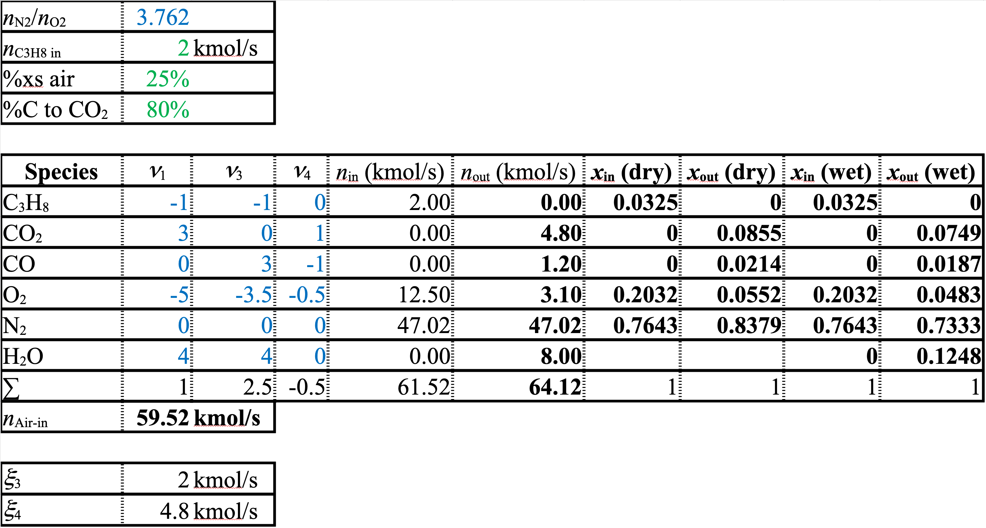
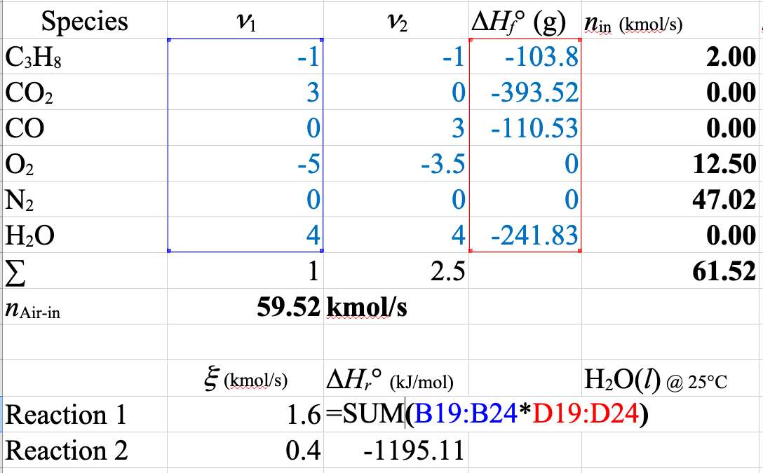
Solution (cont.)
A spreadsheet of the solution for Equation 3 and Equation 4 is shown below
![]()
The stoichiometric coefficients and extents of reaction are different from the first spreadsheet. However, the molar flows and the mole fractions or compositions are identical to those in the version with Equation 1 and Equation 2. As long as you set up a linearly independent balanced set of equations that uses all of the species, it doesn’t matter what set you use. The flows and compositions will all come out the same.
Solution (cont.)
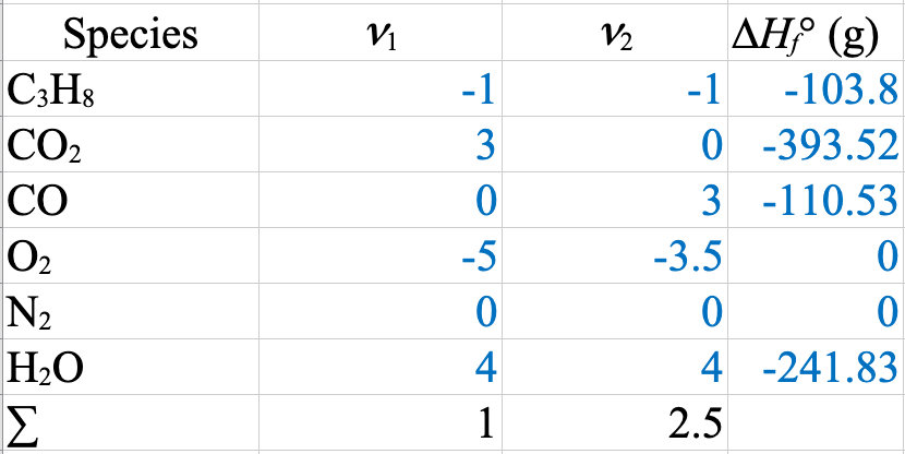
We will finish React Hard: The First Law Gets Chemical with heat-of-reaction with extent of reaction method for Equation 1 and Equation 2.
In React Harder: Formation Heats and Alternate Endings we’ll do the heat of reaction and extent of reaction method for Equation 3 and Equation 4. and compare the answers.
\[\sum\limits_{\substack{\mathrm{out} \\ \mathrm{streams}}} \dot{n}_j \hat{H}_j\ - \sum\limits_{\substack{\mathrm{in} \\ \mathrm{streams}}} \dot{n}_i \hat{H}_i + \sum\limits_\mathrm{rxns} \dot{\xi}_k \left( \Delta \hat{H}^\circ_r\right)_k = \dot{Q}\]
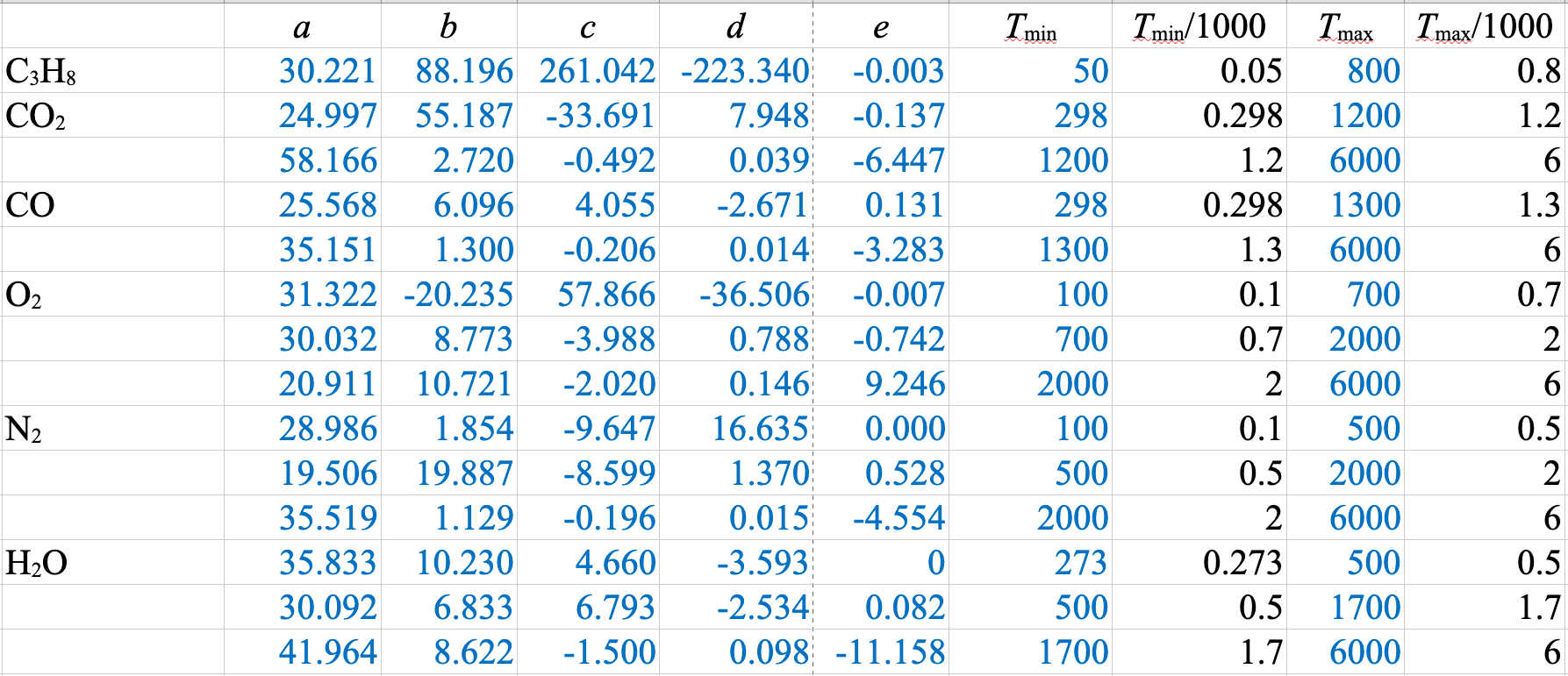
\[\hat{H}_i = \int\limits_{T_\mathrm{ref}}^T C_{pi} (T) dT = \int\limits_{T_\mathrm{ref}}^T (a_i + b_i T + c_i T^2 + d_i T^3 + \dfrac{e_i}{T^2})dT\]
\[\left(\Delta \hat{H}^\circ_r\right)_k = \sum \nu_{ik} \Delta \hat{H}^\circ_{fi}\]
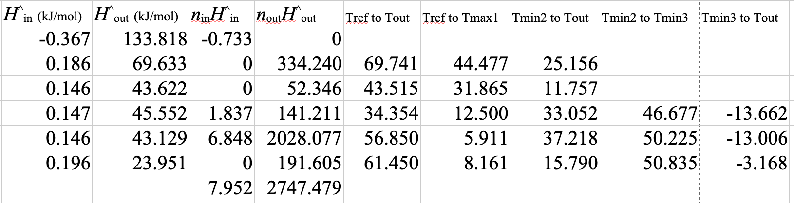
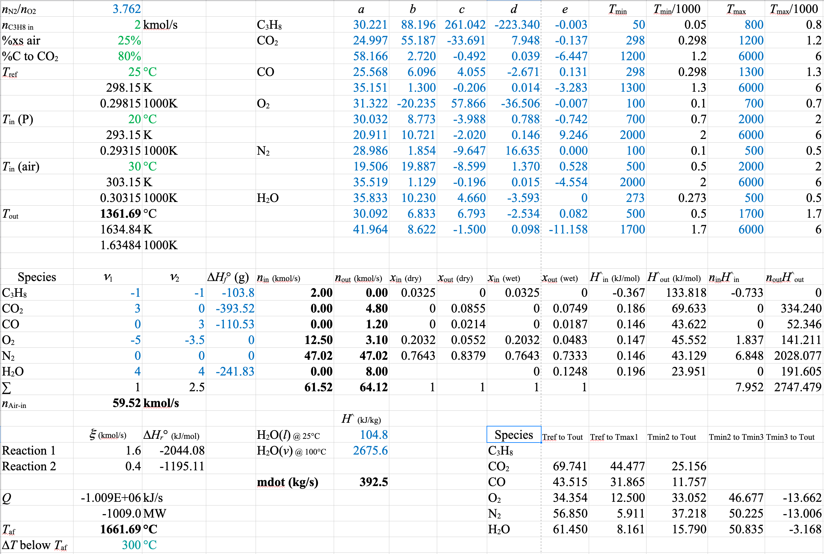
We will finish with the heat-of-formation method.
![]()
\(\dot{m}_\mathrm{H_2O} = \dfrac{-\dot{Q}}{\Delta \hat{H}_\mathrm{H_2O}} = \dfrac{1009 \times 10^3}{2676 - 104.8} = 393\ \mathrm{kg/s}\)
The Takeaways
- It’s good to start with a mole-balance spreadsheet when doing 1st-Law balances on a reacting system.
- Sometimes you have to do piecewise integration on your heat-capacity equations.
- Spreadsheets can help you keep your information organized.