Add Friction and Work to Bernoulli? Here’s What Really Happens!
DOFPro Team
Introduction
- Fluid flowing through:
- A tube
- A pipe
- A culvert
- A sluice
- Not gaining or losing energy through heat transfer other than friction
- The Mechanical Energy Balance
The Mechanical Energy Balance
If we start with the 1st law for an open steady-state system,
\[ \dot{m}\Delta(\hat{U}+P\hat{V})+ \dot{m} \Delta \frac{u^2}{2}+\dot{m}g\Delta z -\dot{Q}=\dot{W}_s \]
and gather the internal energy term with the heat, and assume an incompressible liquid such that
\[ \hat{V} = \frac{1}{\rho}=\mathrm{const}. \]
Then the 1st law becomes
\[ \dot{m} \Delta \frac{P}{\rho} + \dot{m} \Delta \frac{u^2}{2} + \dot{m} g \Delta z + (\dot{m} \Delta \hat{U} - \dot{Q}) = \dot{W}_s \]
The Mechanical Energy Balance (cont.)
or dividing through by the mass flow rate
\[ \Delta \frac{P}{\rho} + \Delta \frac{u^2}{2} + g \Delta z + \left( \Delta \hat{U} - \frac{\dot{Q}}{\dot{m}} \right) = \frac{\dot{W}_s}{\dot{m}} \]
If the only heating is through friction, we can call the term in parentheses, the friction loss
\[ \hat{F} = \Delta \hat{U} - \frac{\dot{Q}}{\dot{m}} \]
and the 1st law becomes
\[ \boxed {\Delta \frac{P}{\rho} + \Delta \frac{u^2}{2} + g \Delta z + \hat{F} = \frac{\dot{W}_s}{\dot{m}}} \]
The Mechanical Energy Balance (cont.)
If there is no friction loss or shaft work input we have
\[ \Delta \frac{P}{\rho} + \Delta \frac{u^2}{2} + g \Delta z = 0 \]
which is the Bernoulli equation, that you may have seen in high-school physics.
For a circular pipe, the friction loss is
\[ \hat{F} = f \frac{L}{D} \frac{u^2}{2} \]
where \(L\) is the length of the pipe, \(D\) is the diameter of the pipe,and \(u\) is the velocity of the fluid. \(f\) is the Moody friction factor and is a function of the Reynolds number.
The Reynolds number
The Reynolds number is an important dimensionless quantity in fluid mechanics. It is the ratio of momentum to viscous forces. For a pipe, it is calculated as
\[ Re = \frac{\rho u D}{\mu} \quad \text{or} \quad Re = \frac{u D}{\nu} \]
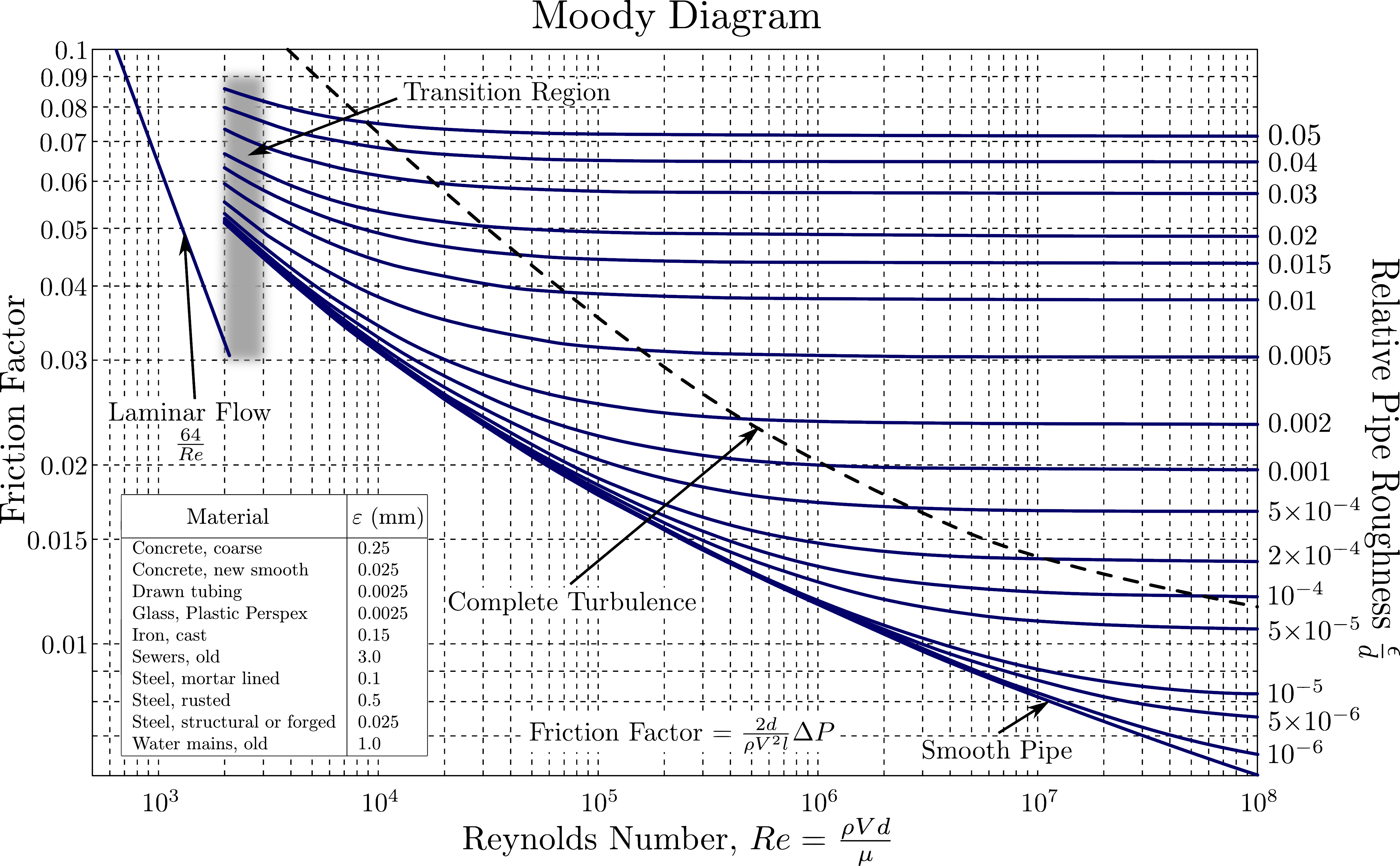
where \(D\) is the diameter of the pipe, \(u\) is the velocity of the fluid, \(\rho\) is the density of the fluid, \(\mu\) is the dynamic viscosity of the fluid, and \(\nu = \mu ⁄ \rho\) , is the kinematic viscosity of the fluid. For \(Re\) < 2100, the flow in the pipe is laminar and \(f = 64⁄Re\). For \(Re > 2300\) , the flow is turbulent, and \(f\) has to be evaluated from a chart called a Moody Chart or Moody Diagram.
Marc.derumaux, CC BY-SA 4.0, via Wikimedia Commons
To use a Moody chart you have to know the Reynolds number and the Surface Roughness of the inside of the pipe. In addition to the Moody (a.k.a Darcy or Blasius) friction factor, there is another friction factor called the Fanning friction factor, It is also given the symbol \(f\). The relationship is
\[ f_\mathrm{Fanning} = f_\mathrm{Moody}/4. \]
Make sure you know which one you are using. Since Wikipedia has a Moody diagram, we’re using the Moody friction factor.
The mechanical energy balance finds extensive use in transport of an incompressible fluid such as water or oil through pipelines, aqueducts, pumps, turbines, and the like.
Example Problem
Water at \(20\ ^\circ\mathrm{C}\) flows at \(0.05\ \mathrm{m^3/s}\) in a \(20\ \mathrm{cm}\) cast iron pipe. Calculate \(\Delta P\) per kilometer.
Properties: \[ \rho = 998 \text{ kg/m}^3, \mu = 1.00 \times 10^{-3} \text{ N s/m}^2. \]
Calculate velocity:
\[ u = \frac{\dot{V}}{A} = \frac{0.05 \text{ m}^3/\text{s}}{\frac{\pi}{4} (0.20 \text{ m})^2} = 1.59 \text{ m/s}. \]
\[ Re = \frac{\rho u D}{\mu} = \frac{998 \text{ kg/m}^3 \cdot (1.59 \text{ m/s}) \cdot 0.20 \text{ m}}{1.00 \times 10^{-3} \text{ N s/m}^2} \]
\(\ \ \ \ \ \ \ \ \ \ \ \ \ \ \ = 3.18 \times 10^5\)
Look up the surface roughness in the table on the Moody Chart.
Marc.derumaux, CC BY-SA 4.0, via Wikimedia Commons
Look up the surface roughness in the table on the Moody Chart.
\[ \varepsilon = 0.15\ \mathrm{mm} \]
The most common mistake is to forget to calculate \(\frac{\varepsilon}{D}\) from \(\varepsilon\).
\[ \frac{\varepsilon}{D} = \frac{0.15 \times 10^{-3} \text{ m}}{0.20 \text{ m}} = 0.00075. \]
Use the Moody Chart (for Moody not Fanning friction factor)
Marc.derumaux, CC BY-SA 4.0, via Wikimedia Commons
\[ f = 0.0195 \]
\[ \hat{F} = f \frac{L}{D} \frac{u^2}{2} = 0.0195 \left( \frac{1000 \text{ m}}{0.2 \text{ m}} \right) \frac{(1.59 \text{ m/s})^2}{2} = 123 \text{ m}^2 / \text{s}^2 \]
Simplify the mechanical energy balance:
\[ \Delta \frac{P}{\rho} + \Delta \frac{u^2}{2} + g \Delta z + \hat{F} = \frac{\dot{W}}{\dot{m}} \]
\[ \Delta P = - \rho \hat{F} = - \left( 998 \frac{\text{kg}}{\text{m}^3} \right) \left( 123 \frac{\text{m}^2}{\text{s}^2} \right) \]
\[ = -123,000 \text{ Pa} = -123 \text{ kPa} = -1.2 \text{ atm} \]
The Takeaways
- For incompressible flow in a pipe, use the mechanical energy balance to calculate the relationship among pressure drop, velocity change, elevation change, and shaft work.
- The mechanical energy balance for flow in a pipe is \(\Delta \frac{P}{\rho} + \Delta \frac{u^2}{2} + g \Delta z + \hat{F} = \frac{\dot{W}_s}{\dot{m}}\).
- Use the Reynolds number, \(Re = \rho u D/\mu\), and the roughness ratio, \(\varepsilon/D\), to find the Moody friction factor on the Moody Chart.
- For no friction and no shaft work, the mechanical energy balance simplifies to the Bernoulli equation, \(\Delta \frac{P}{\rho} + \Delta \frac{u^2}{2} + g \Delta z = 0\).
Thanks for watching!
The previous video in the series is in the link in the upper left. The next video in the series is in the upper right. To learn more about Chemical and Thermal Processes, visit the website linked in the description.
The DOFPro Team
![]()