Sadi Carnot and the Power of Fire, the 1824 Edition Part 1
DOFPro Team

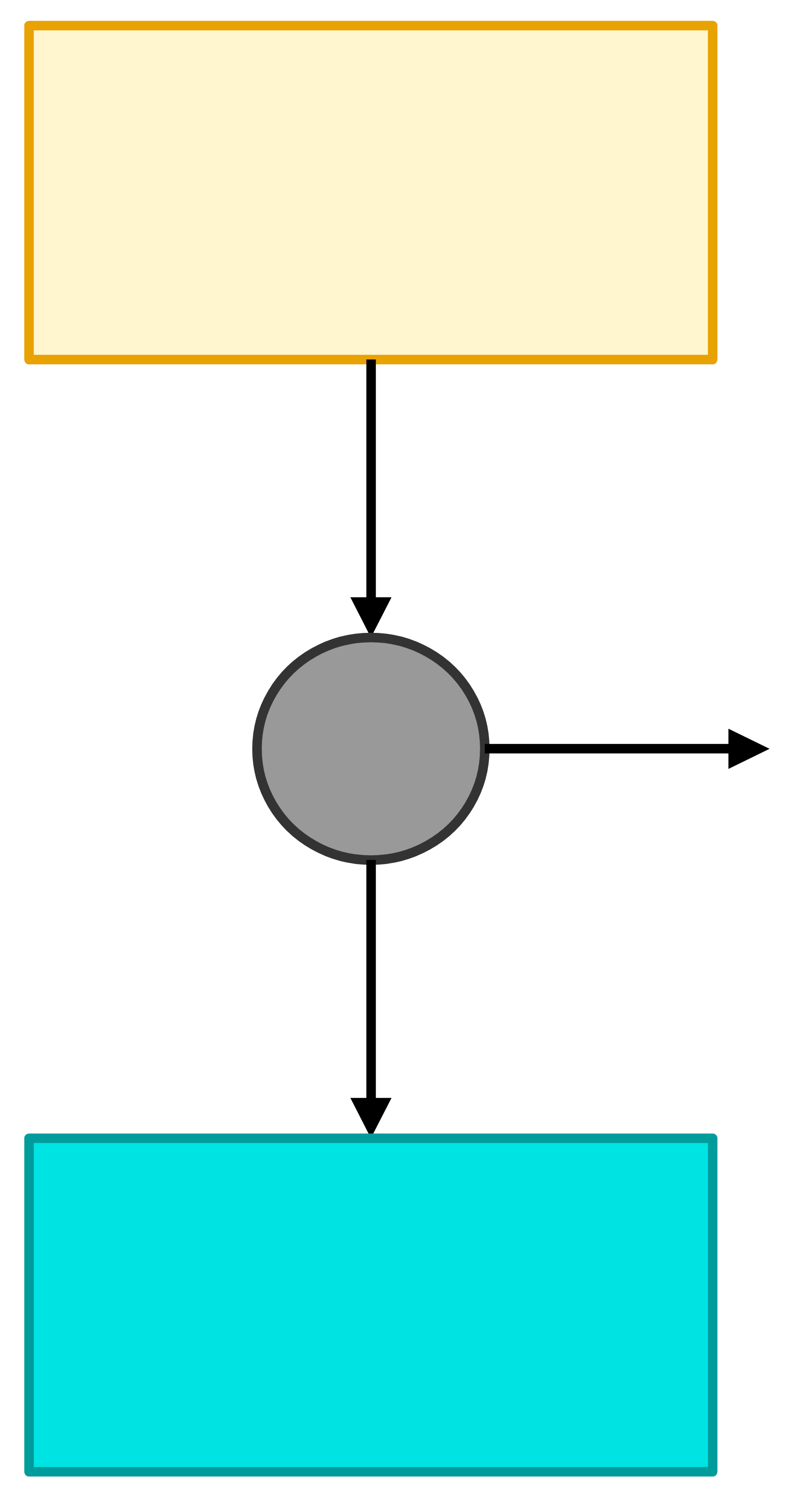
\(T_\mathrm{hot}\)
\(T_\mathrm{cold}\)
\(|Q_\mathrm{hot}|\)
\(|Q_\mathrm{cold}|\)
\(|W|\)
A Carnot engine operates between two isothermal heat reservoirs and produces the greatest possible work while rejecting the minimum amount of heat. The efficiency of a Carnot engine is:
\[\eta \equiv \frac{|W|}{|Q_\mathrm{hot}|} = 1 - \frac{T_\mathrm{cold}}{T_\mathrm{hot}}\]
The four steps of any Carnot engine are:
- Adiabatic temperature change from \(T_\mathrm{cold}\) to \(T_\mathrm{hot}\)
- Isothermal heat addition of \(Q_\mathrm{hot}\) at \(T_\mathrm{hot}\)
- Adiabatic temperature change from \(T_\mathrm{hot}\) to \(T_\mathrm{cold}\)
- Isothermal heat removal of \(Q_\mathrm{cold}\) at \(T_\mathrm{cold}\)
The Complete Cycle
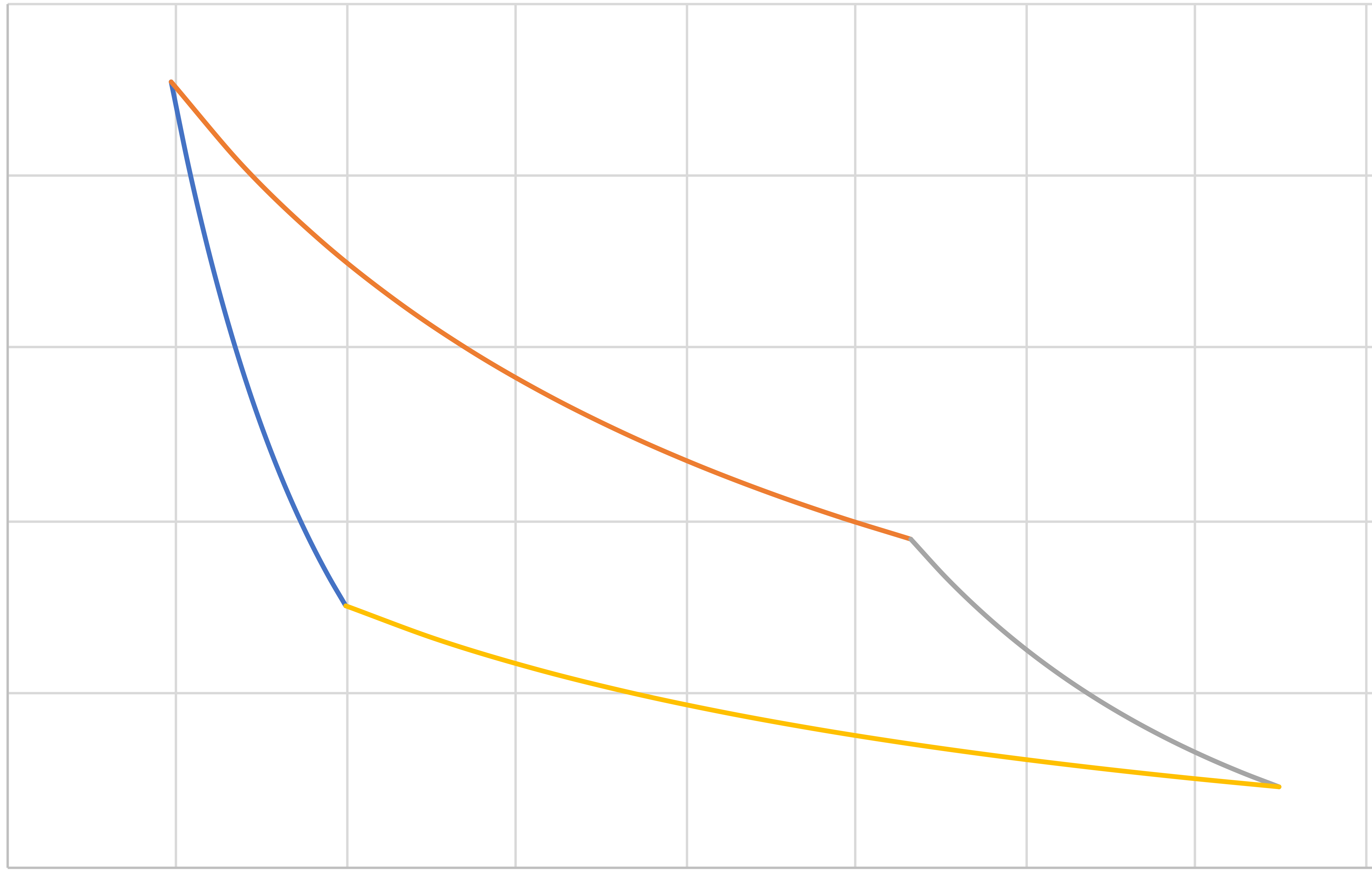
\(a\)
\(b\)
\(c\)
\(d\)
Pressure
Volume
\(PV^\gamma = C_1\)
\(PV = C_2\)
\(PV^\gamma = C_3\)
\(PV = C_4\)
Note that
\(\dfrac{P_b}{P_a} = \left(\dfrac{T_\mathrm{hot}}{T_\mathrm{cold}}\right)^{\frac{C_p}{R}}\)
and
\(\dfrac{P_c}{P_d} = \left(\dfrac{T_\mathrm{hot}}{T_\mathrm{cold}}\right)^{\frac{C_p}{R}}\)
\[\eta = \frac{-W_\mathrm{net}}{Q_\mathrm{hot}} = \frac{R(T_\mathrm{hot} -T_\mathrm{cold}) \ln \dfrac{P_b}{P_c}}{R T_\mathrm{hot} \ln \dfrac{P_b}{P_c}} = \frac{T_\mathrm{hot} - T_\mathrm{cold}}{T_\mathrm{hot}} = 1 - \frac{T_\mathrm{cold}}{T_\mathrm{hot}}\]
Note area enclosed on \(P\hat{V}\) diagram is \(-W_\mathrm{net}\).
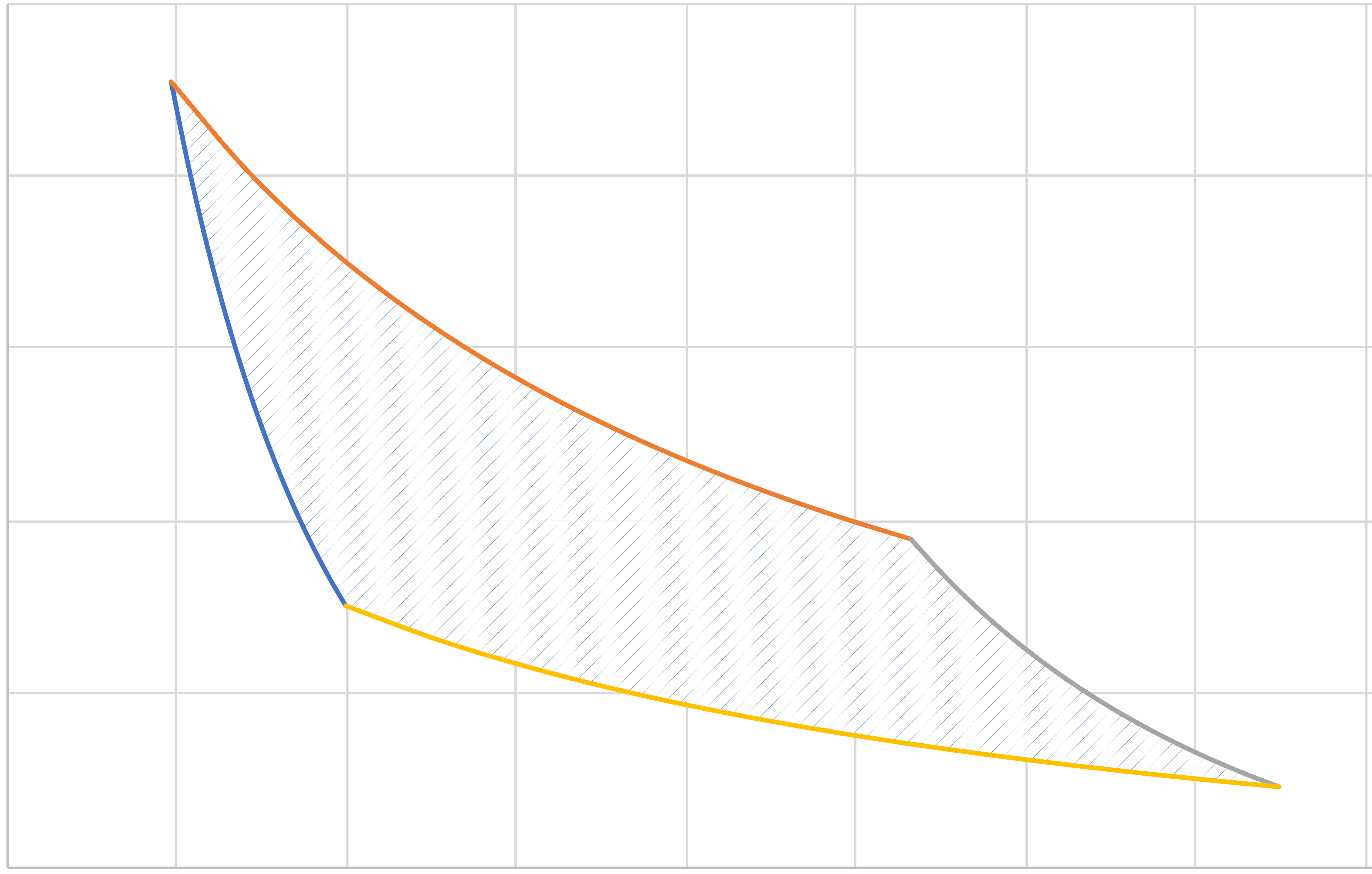
\(a\)
\(b\)
\(c\)
\(d\)
Pressure
Volume
\(PV^\gamma = C_1\)
\(PV = C_2\)
\(PV^\gamma = C_3\)
\(PV = C_4\)
What does a Carnot cycle look like on a \(TS\) diagram?
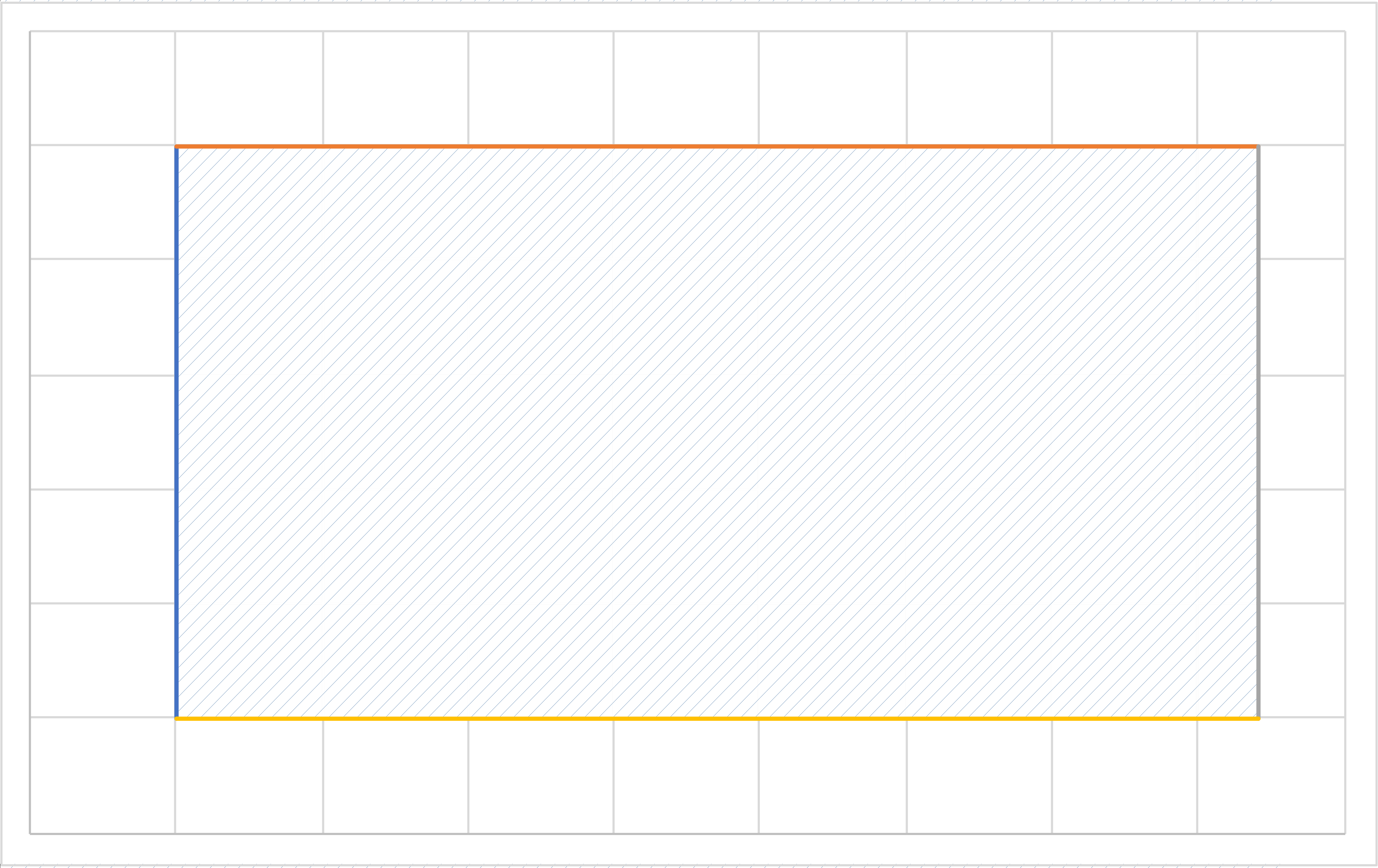
\(\hat{S} = \mathrm{constant}\)
\(T = T_\mathrm{hot}\)
\(\hat{S} = \mathrm{constant}\)
\(T = T_\mathrm{cold}\)
Temperature
Entropy
\(a\)
\(b\)
\(c\)
\(d\)
For cycle
\[-W_\mathrm{net} = Q_\mathrm{net}\]
The Carnot efficiency does not depend on the working fluid.
Thanks for watching!
The previous video in the series is in the link in the upper left. The next video in the series is in the upper right. To learn more about Chemical and Thermal Processes, visit the website linked in the description.
The DOFPro Team