Entropy Made Me Do It: Pumps, Nozzles, and Other Second-Law Shenanigans (Part 2)
![]()
Introduction
These videos, Entropy Made Me Do It, Part 1 and Part 2 derive the equations for common items in power and refrigeration machinery.
- the turbine or expander
- the adiabatic compressor
- the isothermal compressor
- the pump
- the nozzle
- the valve or throttle
Up Third
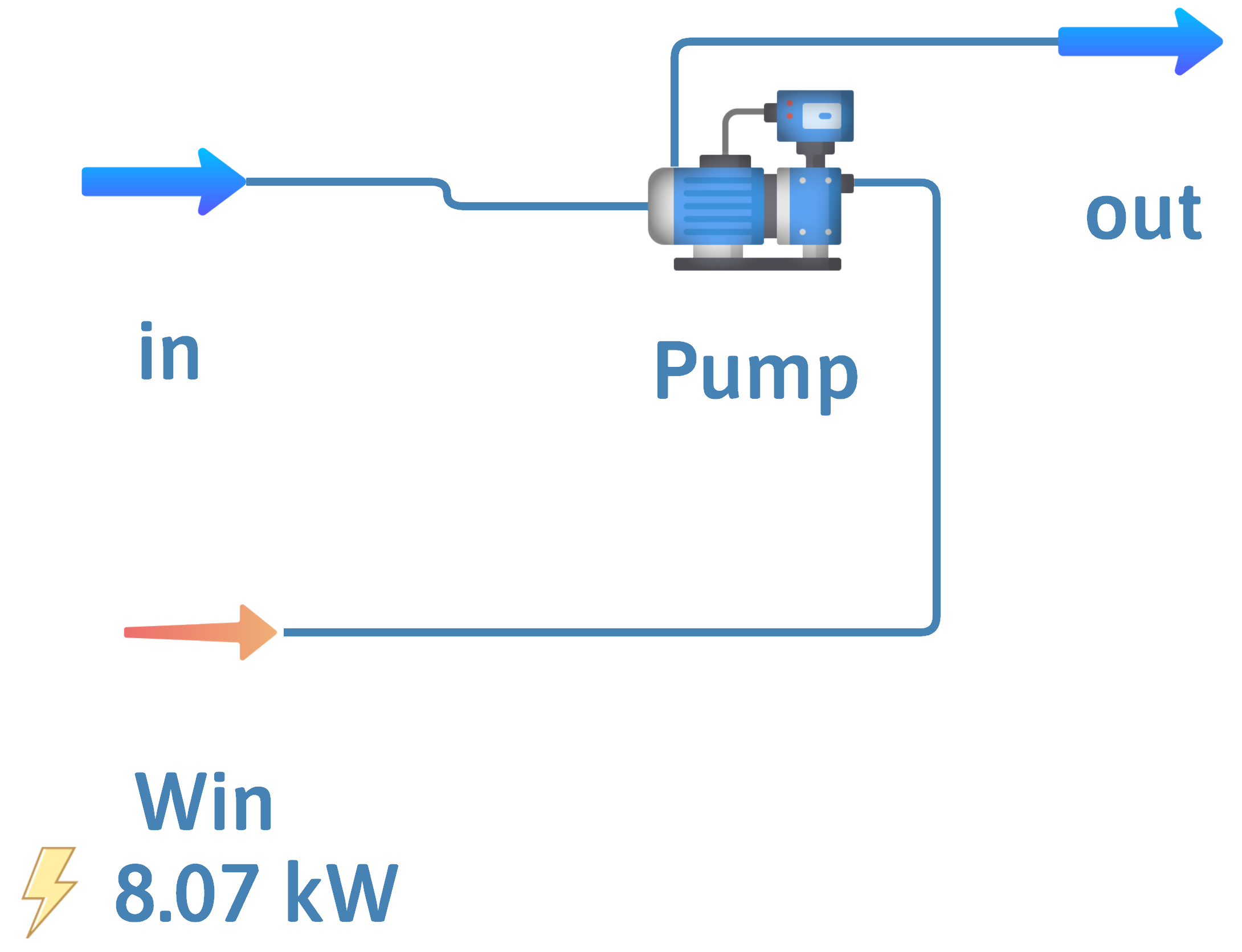
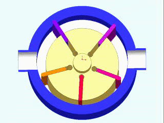
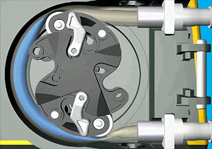
Pump – Incompressible Liquids
![]()
![]()
Inputs – \(\dot{m}\) or \(\dot{n}\), \(T\) and \(P\)
Outputs – \(\dot{m}\) or \(\dot{n}\), \(P\)
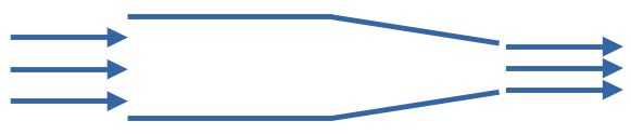
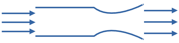
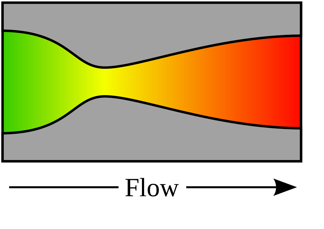
Nozzle – Ideal Gas or Steam
![]()
![]()
Inputs – \(\dot{m}\) or \(\dot{n}\), \(T\) and \(P\)
Outputs – \(\dot{m}\) or \(\dot{n}\), \(P\)
Goal is velocity increase
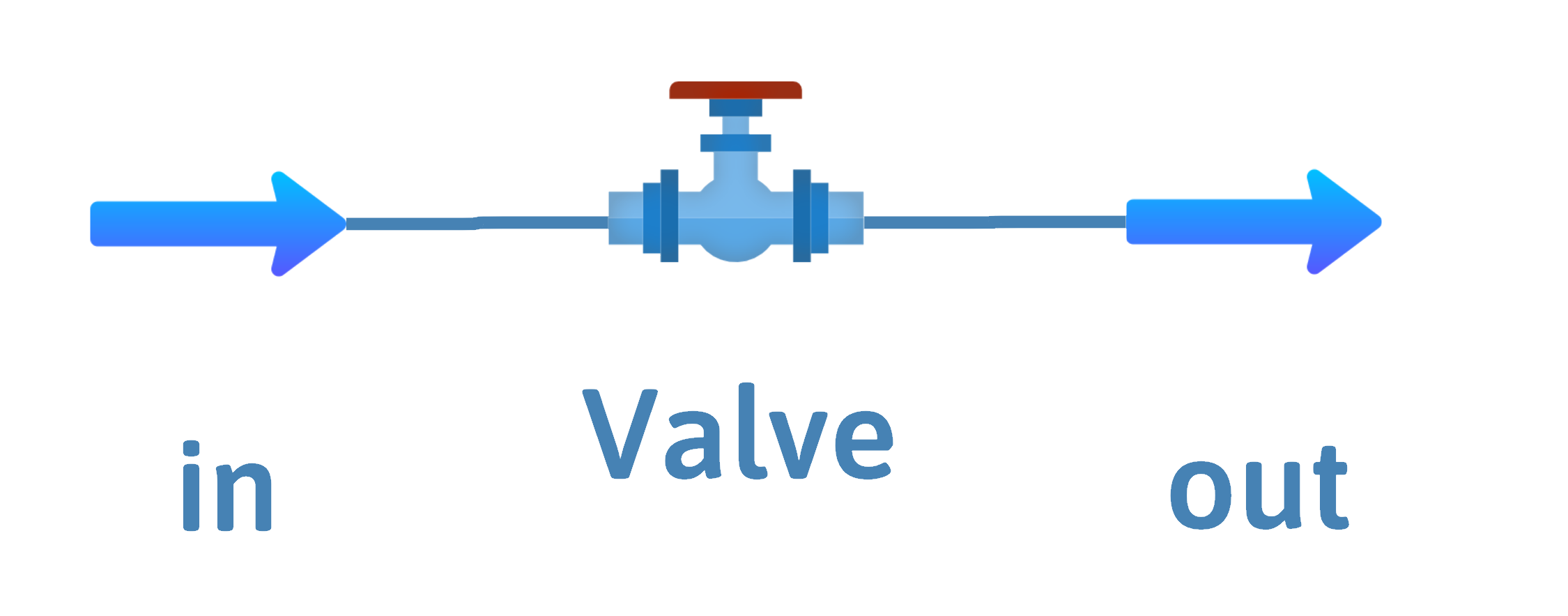
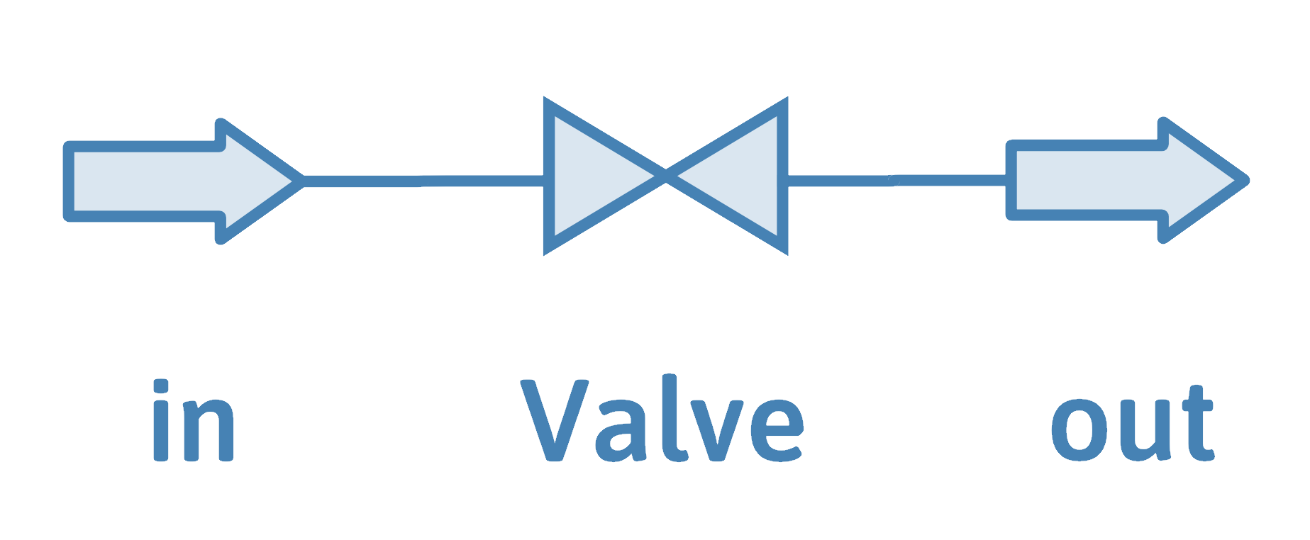
Valve or Throttling Process – Ideal Gas or Two-phase Mixture
![]()
![]()
Inputs – \(\dot{m}\) or \(\dot{n}\), \(T\) and \(P\)
Outputs – \(\dot{m}\) or \(\dot{n}\), \(P\)
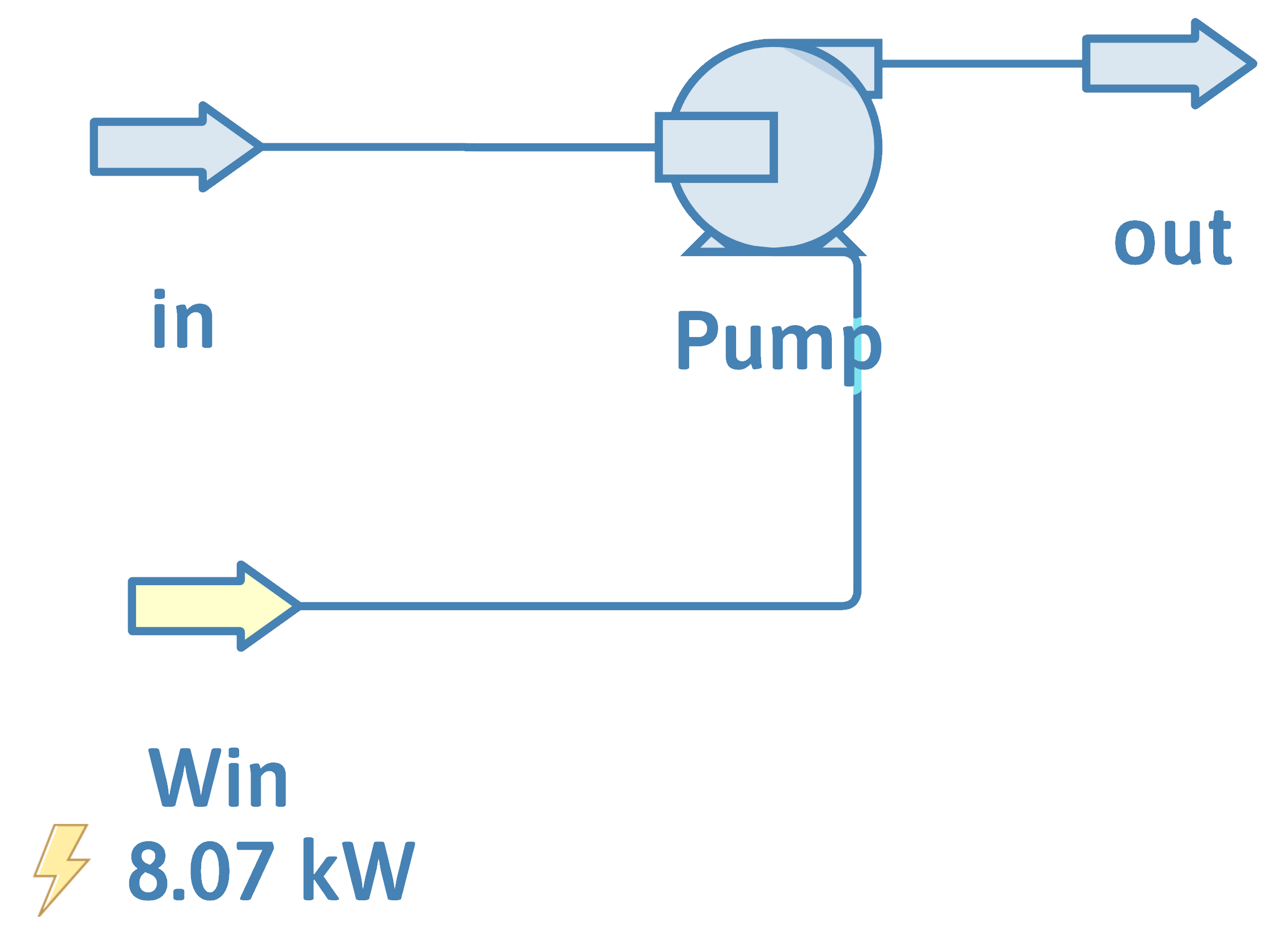
Pump
Incompressible liquid only in introductory videos.
![]()
![]()
Pump
A real pump has a pump efficiency, that compares its performance with that of an isentropic pump.
\[\eta_\mathrm{pump} = \frac{\dot{W}_{s\text{-isentropic}}}{\dot{W}_{s\text{-actual}}} = \frac{\Delta \hat{H}_{\text{isentropic}}}{\Delta \hat{H}_{\text{actual}}}\]
From the fundamental property relationships
\[d\hat{U} = T d\hat{S} - P d\hat{V}\]
\[d\hat{H} = d\hat{U} + P d\hat{V} + \hat{V} dP\ \ \text{from}\ \ \hat{H} = \hat{U} + P \hat{V}\]
\[d\hat{U} = d\hat{H} - P d\hat{V} - \hat{V} dP\]
so
\[d\hat{H} - P d\hat{V} - \hat{V} dP = T d\hat{S} - P d\hat{V}\]
or
\[d\hat{H} = T d\hat{S} + \hat{V} dP\]
Second Law on pump (adiabatic and reversible)
\[d\hat{H} = \hat{V} dP\]
For liquids \(V\) is a very weak function of pressure (hence incompressible).
\[\int d\hat{H} = \int \hat{V} dP = \hat{V} \int dP\]
\[\Delta H_\text{isentropic} = W_{s\text{-isentropic}} = V \Delta P\]
Calculating the actual work
\[\dot{W}_{s\text{-actual}} = \frac{\dot{W}_{s\text{-isentropic}}}{\eta_\mathrm{pump}}\]
\[\Delta \hat{H}_{\text{actual}} = \frac{\Delta \hat{H}_{\text{isentropic}}}{\eta_\mathrm{pump}}\]
If necessary, you can calculate the actual entropy change.
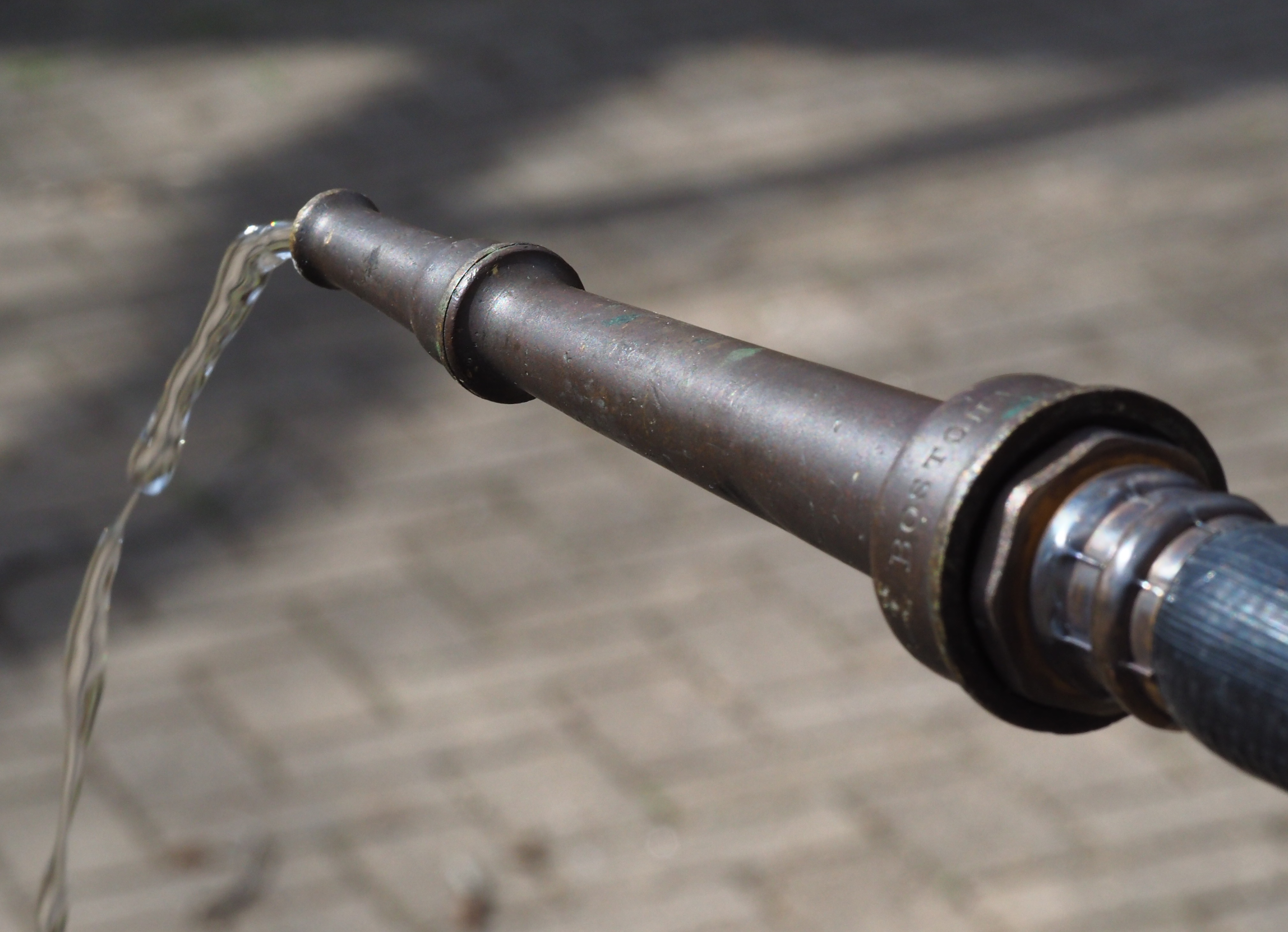
Nozzle
![]()
![]()
No machine-readable author provided. HorsePunchKid assumed (based on copyright claims)., CC BY-SA 3.0, via Wikimedia Commons
Nozzle
A real nozzle has a nozzle efficiency, that compares its performance with that of an isentropic nozzle.
\[\eta_\mathrm{nozzle} = \frac{u^2_{\text{out-actual}}}{u^2_{\text{out-isentropic}}}\]
The point of a nozzle is to get a huge increase in velocity.
\[\Delta \dot{H} + \Delta \dot{E}_\mathrm{k} = 0\]
\[\hat{H}_\mathrm{out} - \hat{H}_\mathrm{in} + \frac{u^2_\mathrm{out}}{2} - \frac{u^2_\mathrm{in}}{2} = 0\]
\[u^2_\mathrm{out} = 2\left(\hat{H}_\mathrm{in} - \hat{H}_\mathrm{out}\right) + u^2_\mathrm{in}\]
\(u_\mathrm{out} = \sqrt{2\left(\hat{H}_\mathrm{in} - \hat{H}_\mathrm{out}\right) + u^2_\mathrm{in}}\ \ \ \ \ \) Be careful with units.
\[\Delta \dot{S} = 0\ \ \ \ \ \ \ \ \hat{S}_\mathrm{out} = \hat{S}_\mathrm{in}\]
\[\Delta \hat{S} = 0 = C_p \ln \frac{T_\mathrm{out}}{T_\mathrm{in}} - R \ln \frac{P_\mathrm{out}}{P_\mathrm{in}}\]
\[C_p \ln \frac{T_\mathrm{out}}{T_\mathrm{in}} = R \ln \frac{T_\mathrm{out}}{T_\mathrm{in}}\ \ \ \ \text{or}\ \ \ \ \frac{T_\mathrm{out}}{T_\mathrm{in}} = \left(\frac{P_\mathrm{out}}{P_\mathrm{in}}\right)^\frac{R}{C_p}\]
Substitute in for \(\Delta T\).
\[\Delta \hat{H}_{\text{actual}} = C_p \Delta T_\text{actual} = C_p \left(T_\mathrm{out} - T_\mathrm{in}\right)\]
\[= C_p T_\mathrm{in}\left[\left(\frac{P_\mathrm{out}}{P_\mathrm{in}}\right)^\frac{R}{C_p} - 1\right]\]
\[u^2_\text{out-isen} - u^2_\text{in} = -2 C_p \Delta T_\text{in} = 2 C_p T_\mathrm{in}\left[1 - \left(\frac{P_\mathrm{out}}{P_\mathrm{in}}\right)^\frac{R}{C_p}\right]\]
For steam find the value of enthalpy in the steam table at the same entropy and pressure as the outlet.
\(u_\text{out-isen} = \sqrt{2\left(\hat{H}_\mathrm{in} - \hat{H}_\mathrm{out}\right) + u^2_\mathrm{in}}\ \ \ \ \) Be careful with units.
For either steam or ideal gas find the actual velocity with the efficiency.
\[u^2_\text{out-actual} = \eta_\mathrm{nozzle}u^2_{\text{out-isentropic}}\]
If necessary, you can calculate the actual temperature, enthalpy change, and entropy change.
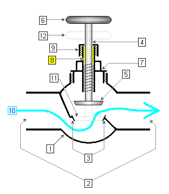
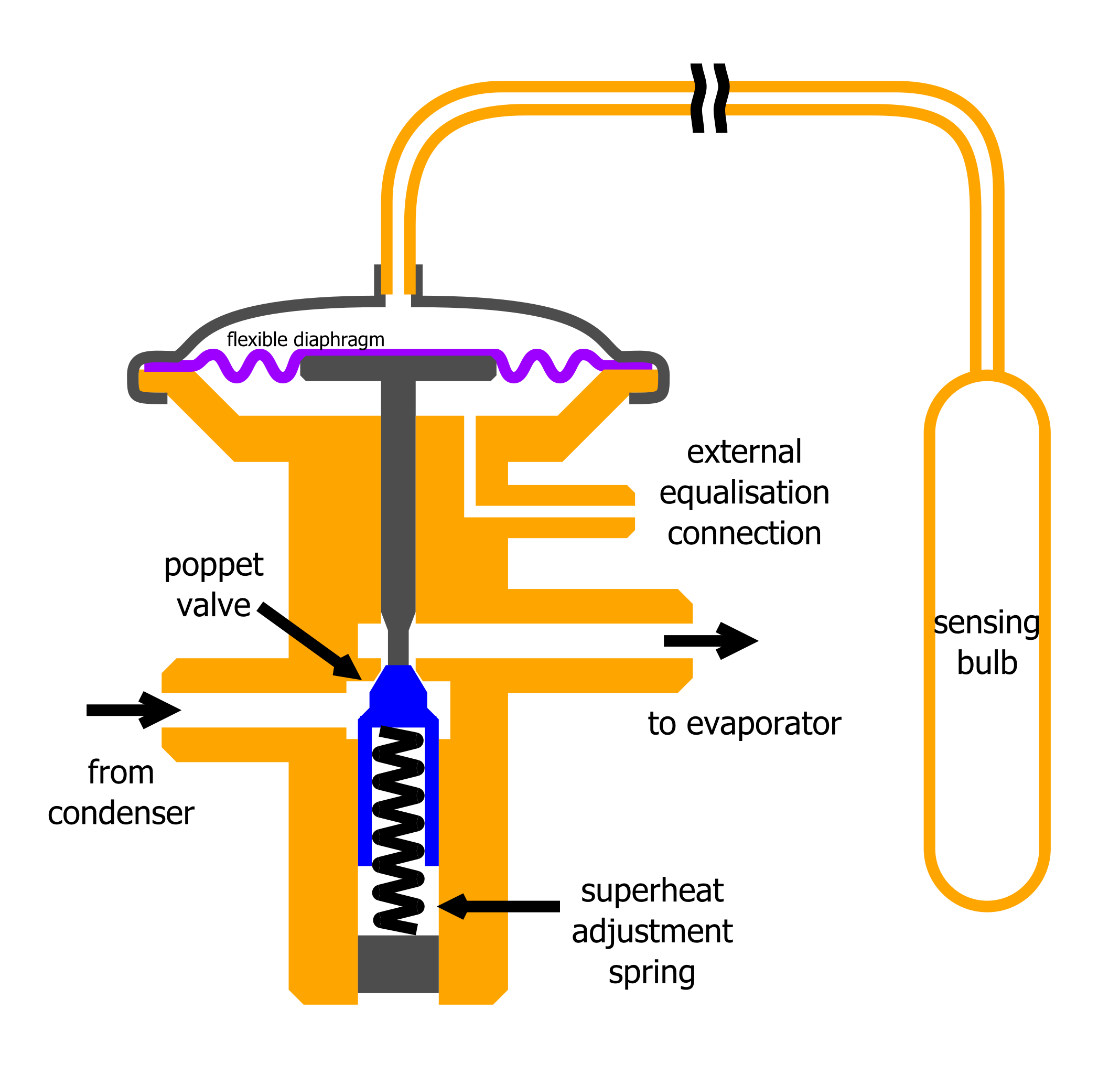
Valves
A partially open valve, an orifice, or a throttling valve can all be described as a throttling process.
![]()
![]()
Throttling Process
Because the fluid passes quickly through a throttling process, the heat transfer is essentially zero. The First Law becomes
\[\Delta \dot{H} + \Delta \dot{E}_\mathrm{k} + \Delta \dot{E}_\mathrm{p} = \dot{Q} + \dot{W}_s\]
\[\hat{H}_\mathrm{out} = \hat{H}_\mathrm{in}\]
There isn’t much to a throttling process for an ideal gas, since the enthalpy is a function of temperature and \(\Delta H = 0\), so \(\Delta T = 0\).
\[P_\mathrm{out} \hat{V}_\mathrm{out} = P_\mathrm{in} \hat{V}_\mathrm{in}\]
Throttling Process (cont.)
A throttling process for a liquid at the edge of the two-phase region is much more interesting. Normally, one specifies the inlet \(T\) and \(P\), that the quality in, \(x = 0\), and the outlet \(P\).
\[\hat{H}_\mathrm{out} = \hat{H}_\mathrm{in}\]
One then uses the fluid two-phase table to determine the final pressure and quality.
For example, take saturated liquid water at 50 bar, and flash it to 1 bar. Calculate the final \(T\) and \(x\).
Throttling Process Example
At \(50\ \mathrm{bar}\) and \(263.94\ ^\circ \mathrm{C}\)
\[\hat{H}_\mathrm{in} = 1154.5\ \mathrm{kJ/kg}\]
\[T_\mathrm{out} = 99.61\ ^\circ \mathrm{C}\]
\[\hat{H}_l = 417.44\ \mathrm{kJ/kg}\ \ \ \ \ \ \hat{H}_v = 2674.9\ \mathrm{kJ/kg}\]
\[\Delta \hat{H}_{lv} = 2257.5\ \mathrm{kJ/kg}\]
\[x = \frac{\hat{H}_\mathrm{out} - \hat{H}_l}{\hat{H}_v - \hat{H}_l} = \frac{1154.5 - 417.44}{2674.9 - 417.44} = 0.3265 = 32.65\%\]
The Takeaways
- Pumps and nozzles all have efficiencies that compare the real or actual case with the isentropic case.
- Valves or throttles have such large irreversibilities that no efficiency is calculated.
- We modeled pumps for incompressible fluids only.
- Nozzles and throttles were modeled for both steam and ideal gas.