Boil, Expand, Condense, Repeat: The Rankine Cycle in Action Part 1

Introduction

Boil, Expand, Condense, Repeat: The Rankine Cycle in Action Part 1 and Part 2

• Describe the Rankine cycle
  • Basic steam power plant cycle
  • Large electrical generating facilities
  • Coal
  • Natural gas
  • Nuclear energy
• Part 1 – The ideal cycle
• Part 2 – Real behavior & DWSIM models

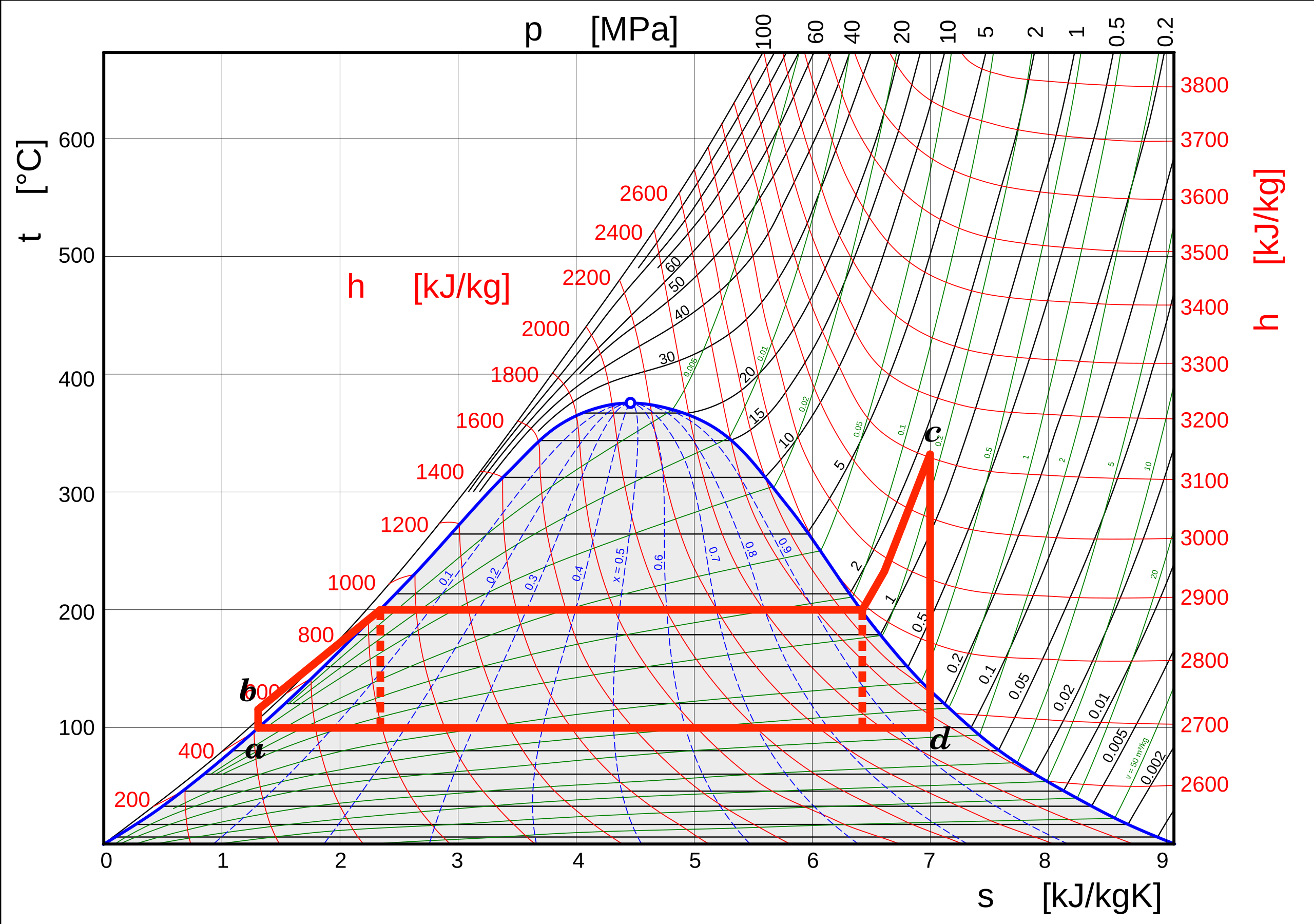
Carnot Steam Cycle

\(a\)

\(b\)

\(c\)

\(d\)

Carnot Steam Cycle

\(a\)

\(b\)

\(c\)

\(d\)

Summary

\[\eta=1-\frac{T_\mathrm{cold}}{T_\mathrm{hot}}=1-\frac{373.15}{473.15}=0.2113\]

\[-W_\mathrm{net}=410.0\ \mathrm{kJ/kg}\]

\[Q_\mathrm{hot}=1939.8\ \mathrm{kJ/kg}\]

\[Q_\mathrm{cold}=-1529.8\ \mathrm{kJ/kg}\]

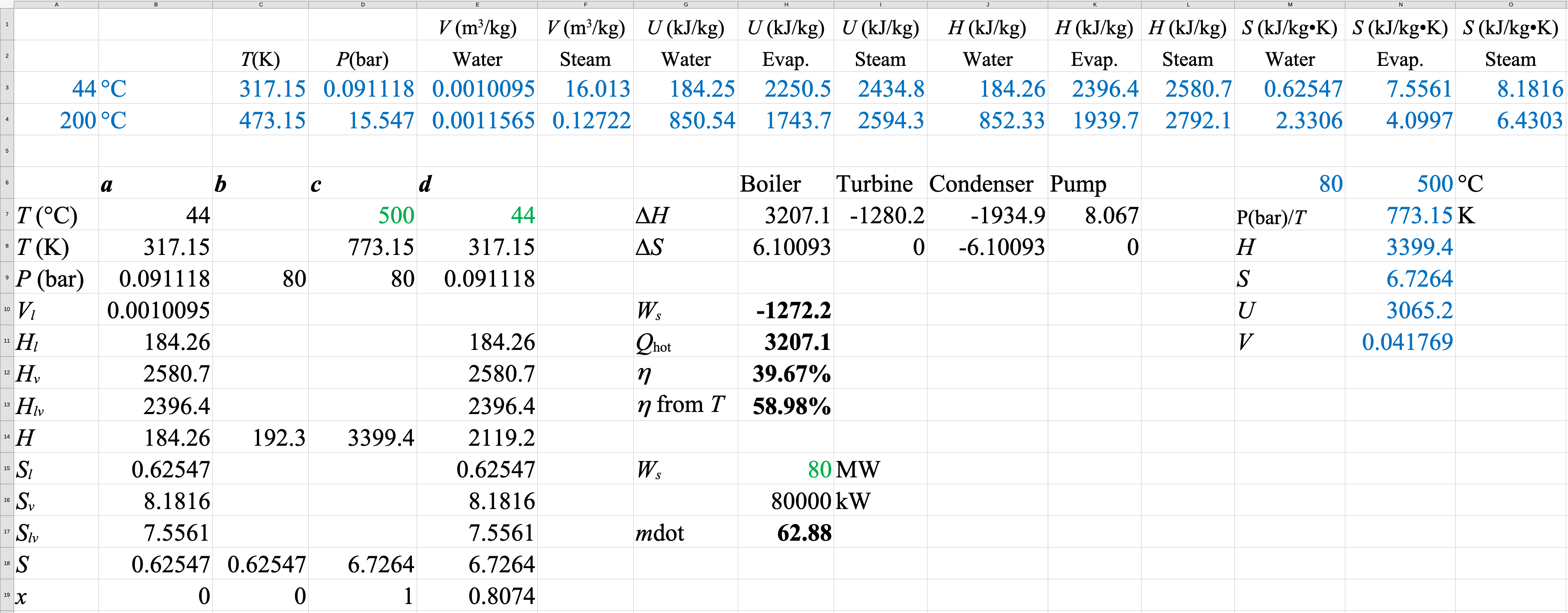
Spreadsheet

What are the engineering problems with the Steam Carnot cycle?

The Rankine Cycle

The Rankine Cycle

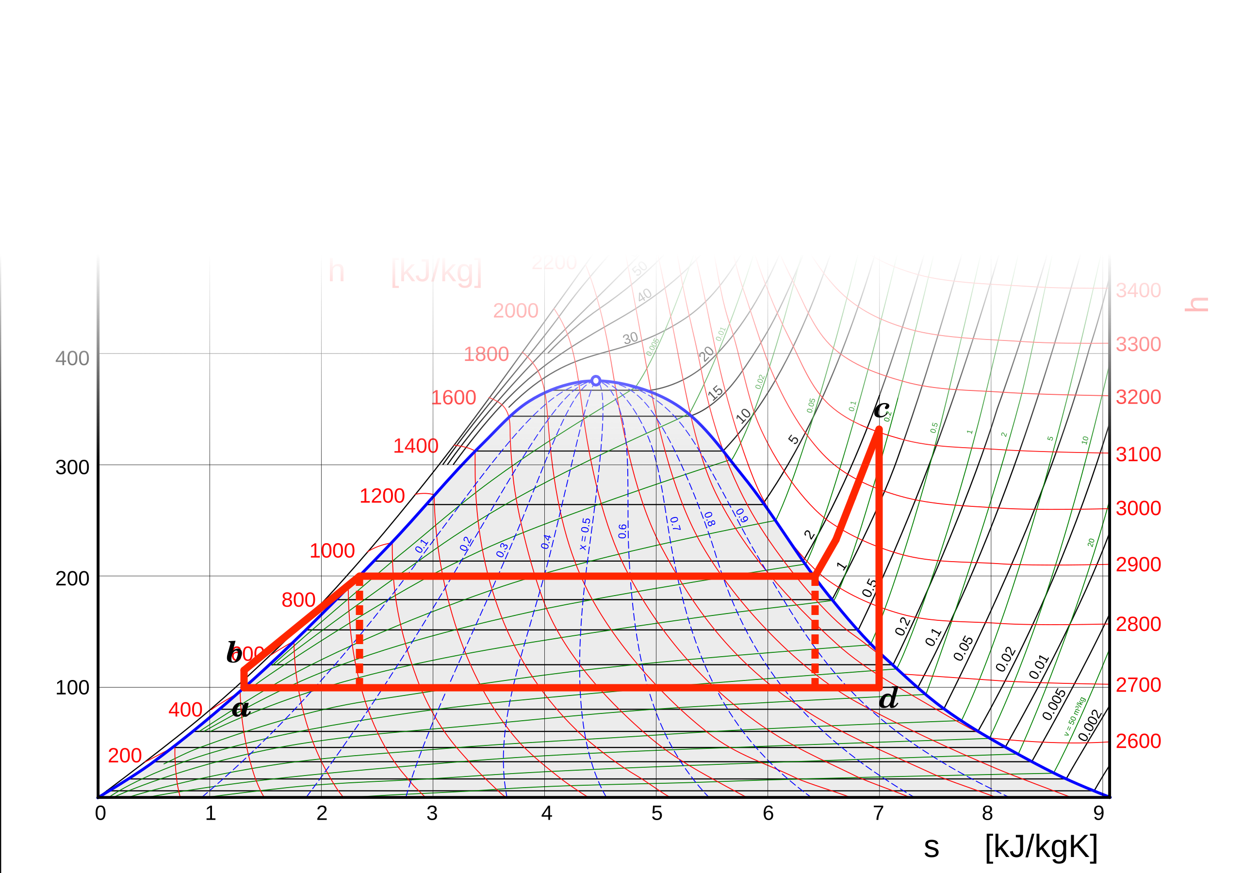
The process from b to c is now
isobaric instead of isothermal.

Pump from a
to b now only
compresses
liquid.

\(\Delta H_\mathrm{pump}=W_{s}=V\Delta P\)

Rankine Cycle Example

A steam power plant operates with steam entering the turbine at 80 bar and 500\(^{\circ}\)C. The condenser operates at 44\(^{\circ}\)C.

1. Calculate the thermal efficiency.
2. What is the water circulation rate for a net power generation of 80 MW?

Data needed from the steam tables:

@ 44\(^{\circ}\)C and 0.091118 bar: \(\hat{H}_{l}\), \(\hat{H}_{v}\), \(\hat{S}_{l}\), \(\hat{S}_{v}\), \(\hat{V}_{l}\)

@ 500\(^{\circ}\)C and 80 bar: \(\hat{H},\hat{S}\)

At 44\(^{\circ}\)C and 0.091118 bar

\(\hat{V_{l}}=0.0010095\mathrm{\frac{m^{3}}{kg}}\) \(\quad\) \(\hat{H}_{l}=184.26\mathrm{\frac{kJ}{kg}}\) \(\quad\) \(\hat{H}_{v}=2580.7\mathrm{\frac{kJ}{kg}}\)

\(\hspace{20cm}\) \(\hat{S}_{l}=0.62547\mathrm{\frac{kJ}{kg~K}}\) \(\quad\) \(\hat{S}_{v}=8.1816\mathrm{\frac{kJ}{kg~K}}\)

At 500\(^{\circ}\)C and 80 bar

\(\hat{H}=3399.4\mathrm{\frac{kJ}{kg}}\)

\(\hat{S}=6.7264\mathrm{\frac{kJ}{kg~K}}\)

Pump

\[\frac{\dot{W_{s}}}{\dot{m}}=\Delta\hat{H}=\hat{V}\Delta P\]

\[=0.0010095\mathrm{\frac{m^{3}}{kg}}(8000\mathrm{~kPa}-9.1118\mathrm{~kPa})=8.067\mathrm{\frac{kJ}{kg}}\]

\[\hat{H}_\mathbf{b}=\hat{H}_\mathbf{a}+\Delta\hat{H}=184.26\mathrm{\frac{kJ}{kg}}+8.067\mathrm{\frac{kJ}{kg}}=192.3\mathrm{\frac{kJ}{kg}}\]

Boiler

\[\Delta\hat{H}=\frac{\dot{Q}}{\dot{m}}=\hat{H}_\mathbf{c}-\hat{H}_\mathbf{b}=3399.4\mathrm{\frac{kJ}{kg}}-192.3\mathrm{\frac{kJ}{kg}}=3207.1\mathrm{\frac{kJ}{kg}}\]

Turbine

\[\frac{\dot{W_{s}}}{\dot{m}}=\Delta\hat{H}\]

\[\Delta\hat{S}=0\Rightarrow\hat{S}_\mathbf{c}=\hat{S}_\mathbf{d}\]

\[6.7264=x(8.1816)+(1-x)(0.62547) \quad x=\frac{6.10093}{7.5561}=0.8074\]

\[\hat{H}_\mathbf{d}=x\hat{H}_{v}+(1-x)\hat{H}_{l}\]

\[=0.8074(2580.7\mathrm{\frac{kJ}{kg}})+(1-0.8074)(184.26\mathrm{\frac{kJ}{kg}})=2119.2\mathrm{\frac{kJ}{kg}}\]

\[\Delta\hat{H}=2119.2\mathrm{\frac{kJ}{kg}}-3399.4\mathrm{\frac{kJ}{kg}}=-1280.2\mathrm{\frac{kJ}{kg}}\]

Efficiency

\[\eta=\frac{-W_\mathrm{net}}{Q_\mathrm{hot}}=\frac{1280.2\mathrm{\frac{kJ}{kg}}-8.067\mathrm{\frac{kJ}{kg}}}{3207.1\mathrm{\frac{kJ}{kg}}}=0.3967=39.7\%\]

Flow Rate

\[-\dot{W}_\mathrm{net}=80,000\mathrm{\frac{kJ}{s}}=-\dot{m}W_\mathrm{net}\]

\[\dot{m}=\frac{-\dot{W}_\mathrm{net}}{-W_\mathrm{net}}=\frac{80,000\mathrm{\frac{kJ}{s}}}{1280.2\mathrm{\frac{kJ}{kg}}-8.067\mathrm{\frac{kJ}{kg}}}=62.88\mathrm{\frac{kg}{s}}\]

Spreadsheet

The Takeaways

1. The ideal Rankine cycle modifies the steam Carnot cycle by fully condensing the water, pumping it, and replacing the isothermal boiler with an isobaric boiler.
2. Compared to the Carnot cycle, the ideal Rankine cycle has a reduced thermal efficiency, but an increased lifetime for the pump and the turbine.
3. As with all power cycles, the thermal efficiency, \(\eta\), is \(|W_\mathrm{net}|\) over \(|Q_\mathrm{hot}|\).

Thanks for watching!
The previous video in the series is in the link in the upper left. The next video in the series is in the upper right. To learn more about Chemical and Thermal Processes, visit the website linked in the description.

The DOFPro Team