Boil, Expand, Condense, Repeat: The Rankine Cycle in Action Part 2
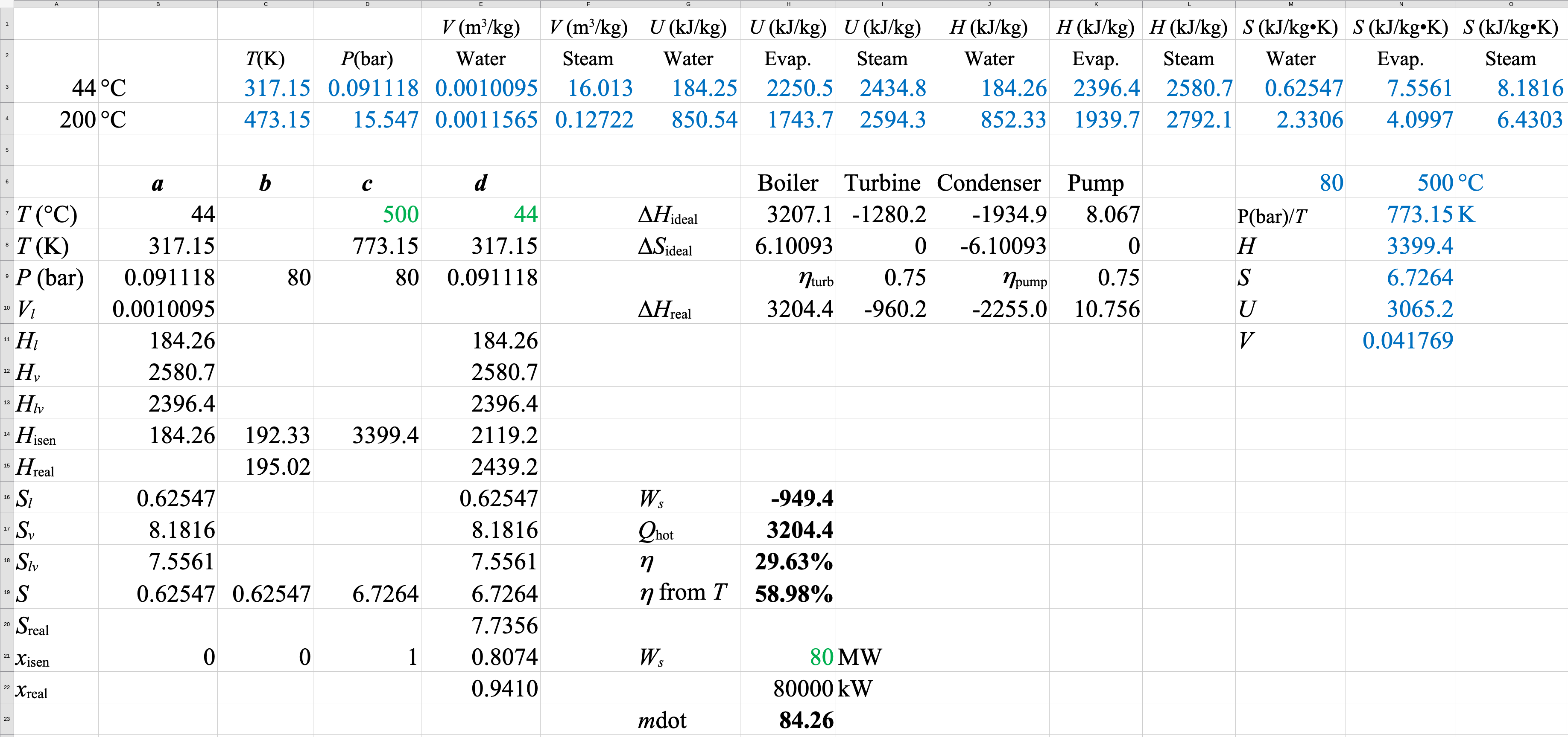
Introduction

Boil, Expand, Condense, Repeat: The Rankine Cycle in Action Part 1 and Part 2

  • Describe the Rankine cycle
    • Basic steam power plant cycle
    • Large electrical generating facilities
    • Coal
    • Natural gas
    • Nuclear energy
  • Part 1 – The ideal cycle
  • Part 2 – Real behavior & DWSIM models

Up the Realism

A more realistic Rankine cycle would include a turbine efficiency and a pump efficiency.

\[\dot{W}_{s–\mathrm{actual}}=\eta_\mathrm{turbine}\dot{W}_{s–\mathrm{isentropic}}\]

\[\dot{W}_{s–\mathrm{actual}}=\frac{\dot{W}_{s–\mathrm{isentropic}}}{\eta_\mathrm{pump}}\]

Realistic Rankine Cycle Example

A steam power plant operates with steam entering the turbine at 80 bar and 500\(^{\circ}\)C. The condenser operates at 44\(^{\circ}\)C. The turbine efficiency, \(\eta_\mathrm{turb}\), and the pump efficiency, \(\eta_\mathrm{pump}\), are both 75%

  1. Calculate the thermal efficiency.
  2. What is the water circulation rate for a net power generation of 80 MW?

Data needed from the steam tables:

@ 44\(^{\circ}\)C and 0.091118 bar: \(\hat{H}_{l}\), \(\hat{H}_{v}\), \(\hat{S}_{l}\), \(\hat{S}_{v}\), \(\hat{V}_{l}\)

@ 500\(^{\circ}\)C and 80 bar: \(\hat{H},\hat{S}\)

Up the Realism (cont.)

Turbine

\[\Delta\hat{H}_\mathrm{ideal}= W_\mathrm{turb–isen}=2119.2\mathrm{\frac{kJ}{kg}}-3399.4\mathrm{\frac{kJ}{kg}}=-1280.2\mathrm{\frac{kJ}{kg}}\]

\[W_\mathrm{turb–real} = \Delta\hat{H}_\mathrm{real} = (\eta_\mathrm{turb})(W_\mathrm{turb–isen})\]

\[= (0.75)(-1280.2)=-960.2\mathrm{\frac{kJ}{kg}}\]

\[\Delta \hat{H}_\mathrm{real} = \hat{H}_\mathbf{d–\mathrm{real}} - \hat{H}_\mathbf{c}\]

\[\hat{H}_\mathbf{d–\mathrm{real}} = \hat{H}_\mathbf{c} + \Delta\hat{H}_\mathrm{real} =3399.4 + (-960.2) = 2439.2 \mathrm{\frac{kJ}{kg}}\]

\[x_\mathbf{d} = \frac{\hat{H}_{\mathbf{d}\mathrm{–real}} - \hat{H}_l}{\hat{H}_v - \hat{H}_l} = \frac{2439.2 - 184.26}{2580.7 - 184.26} = 0.9411\]

Pump

\[W_\mathrm{pump–real} = \Delta\hat{H}_\mathrm{real} = \frac{W_\mathrm{pump–isen}}{\eta_\mathrm{pump}} = \frac{8.067}{0.75}=10.756\mathrm{\frac{kJ}{kg}}\]

\[\hat{H}_\mathbf{b–\mathrm{real}} = \hat{H}_\mathbf{a} + \Delta\hat{H}_\mathrm{real} = 184.26+ 10.756 = 195.02 \mathrm{\frac{kJ}{kg}}\]

Overall

\[W_\mathrm{net–real} = \Delta\hat{H}_\mathrm{turb} +\Delta\hat{H}_\mathrm{pump} = -960.2 +10.76 = -949.4\]

\[Q_\mathrm{hot–real} = \hat{H}_\mathbf{c} - \hat{H}_\mathbf{b–\mathrm{real}} = 3399.4 - 195.02 = 3204.4 \mathrm{\frac{kJ}{kg}}\]

\[\eta_\mathrm{real} = \frac{-W_\mathrm{net–real}}{Q_\mathrm{hot–real}} = \frac{949.4}{3204.4} = 0.2963\ \ \ \text{vs.}\ \ \ \eta_\mathrm{isen} = 0.3967\]

\[\dot{m}=\frac{-\dot{W}_\mathrm{net}}{-W_\mathrm{net}}=\frac{80,000\mathrm{\frac{kJ}{s}}}{960.2\mathrm{\frac{kJ}{kg}}-10.75\mathrm{\frac{kJ}{kg}}}=84.26\mathrm{\frac{kg}{s}}\ \text{vs.}\ 62.88\mathrm{\frac{kg}{s}}\]

Spreadsheet

The Rankine Cycle in DWSIM
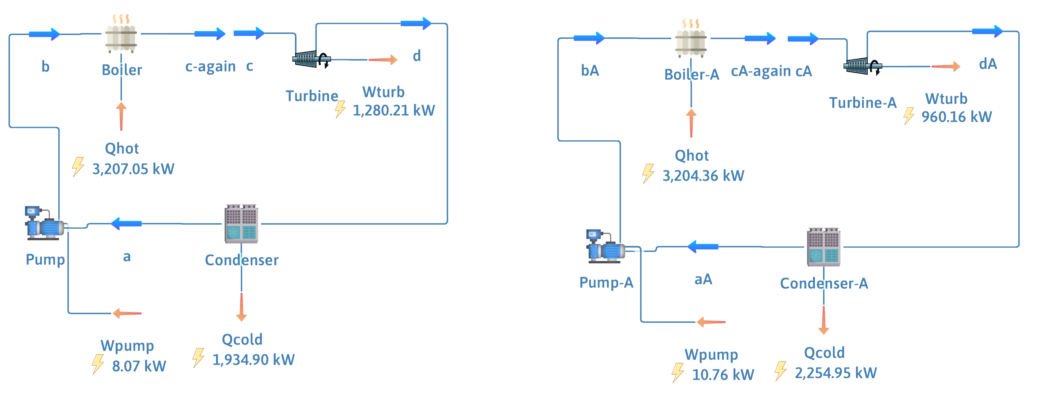
Ideal Cycle

\(\eta = \dfrac{1280.21 - 8.07}{3207.05} = 39.67\%\)

Real Cycle

\(\eta = \dfrac{960.16 - 10.76}{3204.36} = 29.63\%\)

DWSIM Settings


  1. Flow streams c and cA:
    Specified Variables Temperature/Pressure
    Temperature (K) 773.15
    Pressure (Pa) 8000000
    Mass Flow (kg/s) 1
  2. Turbines
    Calculation Mode Outlet Pressure
    Thermodynamic Path Adiabatic
    Outlet Pressure (Pa) 9111.8
    Adiabatic Efficiency (%) 100 or 75
  1. Pumps
    Calculation Mode Outlet Pressure
    Outlet Pressure (Pa) 8000000
    Efficiency (%) 100 or 75
  2. Condensers
    Calculation Mode Outlet Vapor Fraction
    Outlet Vapor Fraction 0
  3. Boilers
    Calculation Mode Outlet Temperature
    Outlet Temperature (K) 773.15

The Takeaways

  1. The calculation of a realistic Rankine cycle starts by doing the calculation for an ideal or isentropic cycle, and adding in the effects of a turbine efficiency and a pump efficiency.
  2. Calculation of the final entropies at the outlet of the turbine, and the outlet of the pump are not necessary for the efficiency calculation. Doing the turbine exit is easy. Doing the pump exit is difficult.
  3. DWSIM has all of the tools necessary to set up and calculate process flow diagrams for Rankine cycles.


Thanks for watching!
The previous video in the series is in the link in the upper left. The next video in the series is in the upper right. To learn more about Chemical and Thermal Processes, visit the website linked in the description.

The DOFPro Team