The Law is a Thief: It Destroys Exergy and Laughs in Your Face Part 2
DOFPro Team

Example
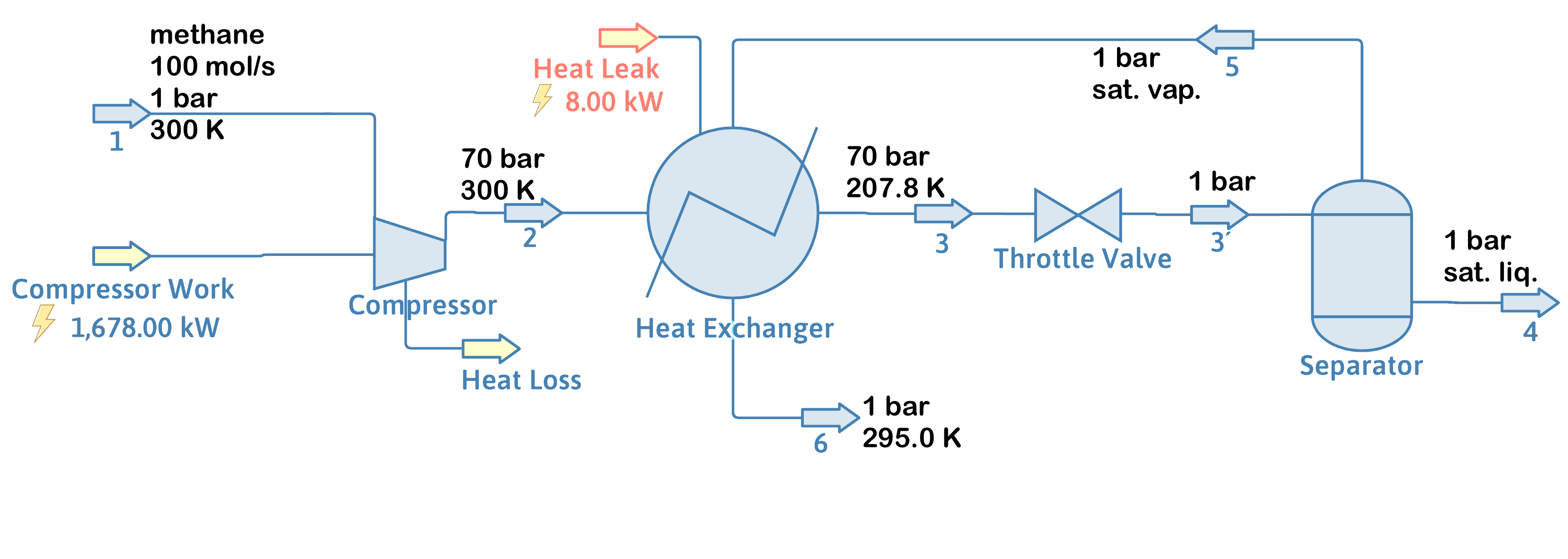
100 moles per second of methane at 300 K and one bar enters the system in Stream 1. It is then compressed and cooled in a multistage compressor with inter- and aftercooling. The unspecified heat from the cooling is rejected to the ambient at \(T_\sigma\) of 300 K. The compressor has a work input of 1678 kilojoules per second or 1678 kilowatts. The methane exits the compressor at 300 K and 70 bar.
The compressed methane then passes through a heat exchanger and exchanges heat with the non-liquified methane from the throttle valve. The compressed methane exits the heat exchanger at 207.8 K and 70 bar. The heat exchanger has a leak of 8 kilojoules per second or 8 kilowatts of heat entering from the ambient at 300 K.
The compressed and cooled methane enters a throttle valve and separator, where it is expanded to one bar and the liquified methane is separated from the still-gaseous methane and sold as LNG or liquified natural gas. The exiting temperature and flow rates have not been specified, but the exiting liquid is in equilibrium with the exiting vapor.
Step 1 – Solve the Mole and Energy Balance
Calculations are done with the CoolProp property package, not Peng-Robinson.
Step 1 (cont.)
Calculations are done with the CoolProp property package, not Peng-Robinson.
Compressor/Cooler
\(\Delta \dot{H} = \dot{Q} + \dot{W}_s\)
\(\dot{Q} = \Delta \dot{H} - \dot{W}_s = \dot{H}_2 - \dot{H}_1 - \dot{W}_s\) \(\ \ \ = 1355.80 - 1466.44 - 1678 = -1789\ \mathrm{kW}\)
Step 1 (cont.)
Calculations are done with the CoolProp property package, not Peng-Robinson.
HX/Valve/Separator
\(\Delta \dot{H} = \dot{Q}\)
\(\dot{H}_4 + \dot{H}_6 - \dot{H}_2 = \dot{Q}\)
\(\dot{m}[(1-x)\hat{H}_4 + x\hat{H}_6 - \hat{H}_2] = \dot{Q}\)
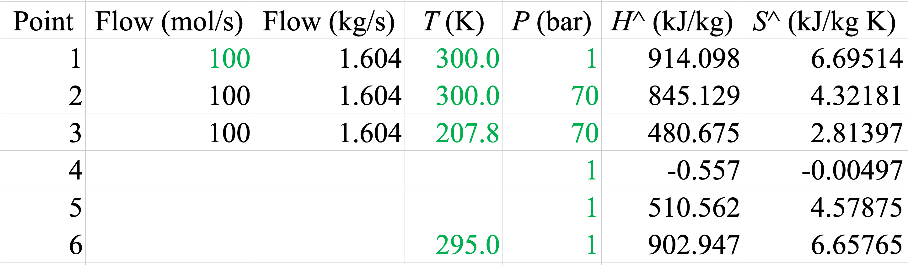
Step 2 – Create Flows and Properties Table
Calculations are done with the CoolProp property package, not Peng-Robinson.
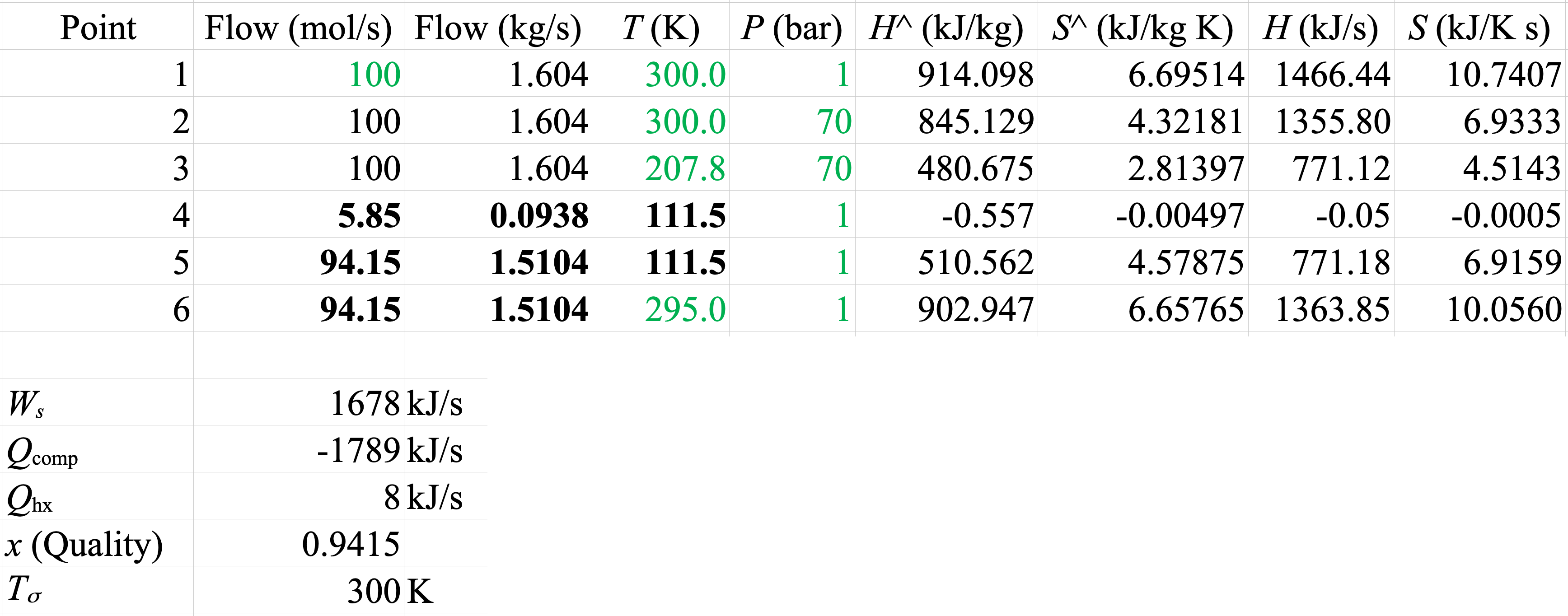
Step 3,4,5 (cont.)
Calculations are done with the CoolProp property package, not Peng-Robinson.
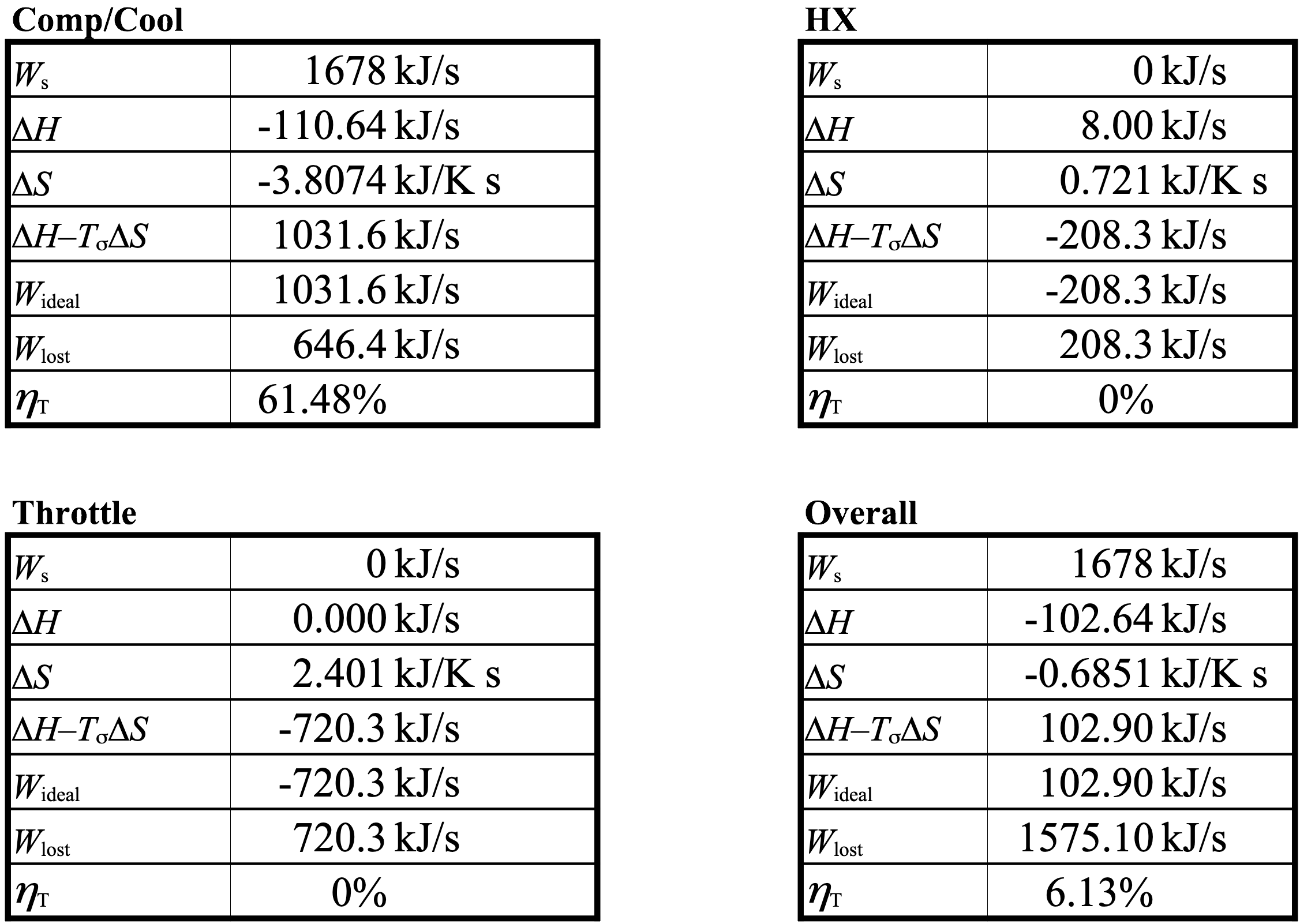
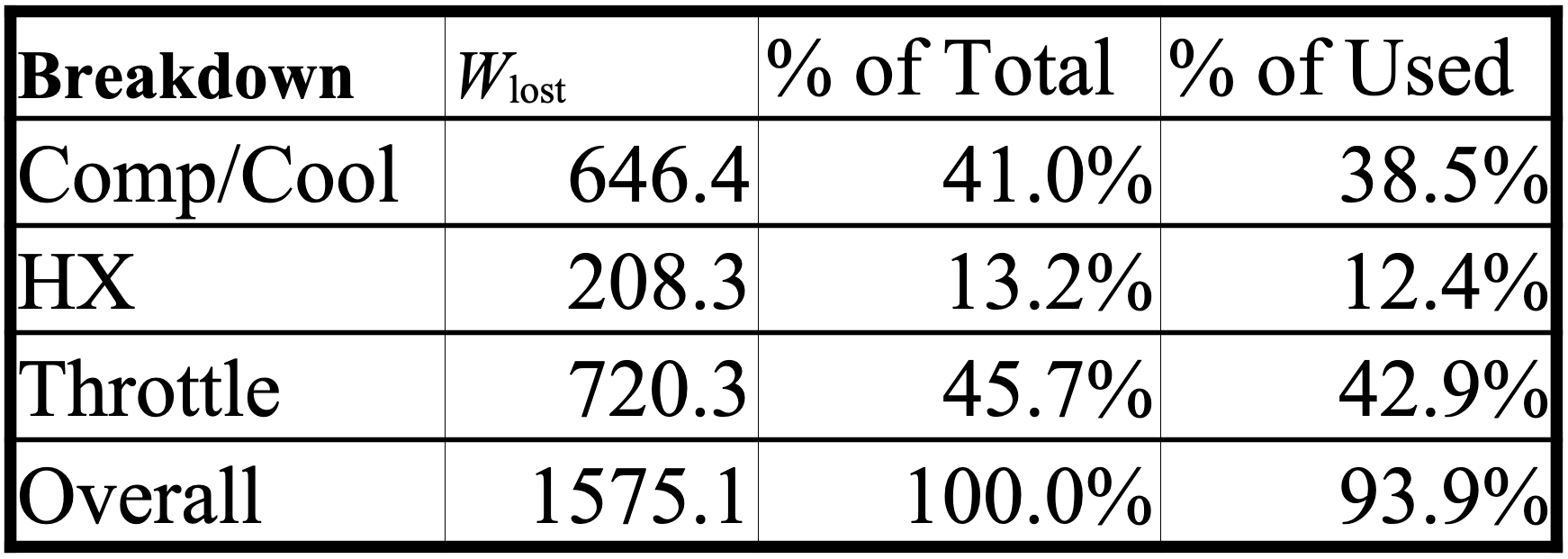
Step 6 – Determine contributions to \(\dot{W}_{\text{lost}}\)
Thanks for watching!
The previous video in the series is in the link in the upper left. The next video in the series is in the upper right. To learn more about Chemical and Thermal Processes, visit the website linked in the description.
The DOFPro Team