Dew Your Bubbles Have Flash? Part 2
DOFPro Team

Dew Your Bubbles Have Flash?
- Use Raoult’s law to perform vapor-liquid phase equilibria calculations.
- Not limited to binaries
- Multicomponent systems conforming to Raoult’s law
- Aliphatic hydrocarbon mixtures
- Aromatic hydrocarbon mixtures
- Part 1 – The basics and BUBL P and DEW P
- Part 2 – BUBL T and DEW T
- Part 3 – FLASH and Pxy and Txy diagrams
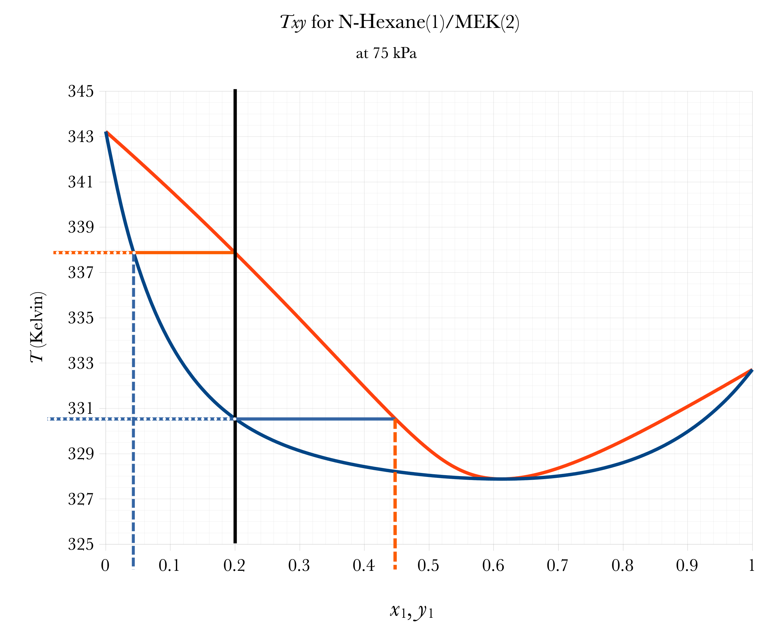
Graphical BUBL T, DEW T
Overall
Composition
Subcooled
Liquid
Superheated
Vapor
\(2\text{–}\phi\)
Dew
Temperature
Dew
Composition
Bubble
Temperature
Bubble
Composition
Low Boiling
Azeotrope
BUBL T
Given all \(x_{i}\)’s and \(P\), calculate \(T\) and \(y_i\)’s
In general, an iterative solution is required. With a spreadsheet, the easiest method is to guess a temperature \(T_\mathrm{guess}\).
Calculate all of the vapor pressures from the Antoine equation, Equation 11,
\[ p_{i}^{*} = 10^{A_{i} - \frac{B_i}{T+C_i}}\ \ \ (i=1,2,3,.., N) \]
Then calculate the pressure from the guessed temperature
\[ P_\mathrm{guess} = \sum_{i=1}^{N} x_{i}p_{i}^{*} \tag{1}\]
Set up a cell to calculate the difference between the actual pressure and the guessed pressure, \(P_\mathrm{actual} - P_\mathrm{guess}\).
Have Goal Seek set the difference to 0 by varying \(T_\mathrm{guess}\).
\(T_\mathrm{guess}\) is now the correct temperature. You can calculate the \(y_i\)’s from Raoult’s law, Equation 12,
\[ y_{i} = \frac{x_{i}p_{i}^{*}}{P}\ \ \ (i=1,2,3,...,N) \]
Alternate Method: In a spreadsheet, guess a \(T\). For one component calculate \(p_{k}^{*}\) from Equation 3 and calculate \(p_{i}^{*}\) from the Antoine equation, Equation 11. Set a cell as the error between the two and goal seek to set that cell to \(0\) by varying \(T\).
Note: For a two-component system, if you are determining the \(y_i\)’s as a function of \(T\) at constant \(P\), you don’t need to iterate. Choose values of \(T\) between \(T_\mathrm{b1}\) and \(T_\mathrm{b2}\), and calculate the \(y_i\)’s using the Antoine equation, Equation 11 and Raoult’s law, Equation 12.
If you prefer programming to spreadsheets, begin by picking an arbitrary component, \(k\), then:
\[ P = p_{k}^{*} \sum_{i=1}^{N} x_{i} \frac{p_{i}^{*}}{p_{k}^{*}} \tag{2}\]
or
\[ p_{k}^{*} = \frac{P}{\sum\limits_{i=1}^{N} x_{i} \alpha_{ik}} \tag{3}\]
where the relative voltatility, \(\alpha_{ik}\), is defined as:
\[ \alpha_{ik} \equiv \frac{p_{i}^{*}}{p_{k}^{*}} \tag{4}\]
If the vapor pressures are related by the Antoine equation, Equation 11:
\[ \log_{10} p^* = A - \frac{B}{T + C} \]
then we can calculate,
\[ \log_{10}\alpha_{ik} = A_i - A_k - \frac{B_i}{T + C_i} + \frac{B_k}{T + C_k} \tag{5}\]
One can begin the iteration with an initial guess
\[ T_{0} = \sum_{i=1}^{N} x_{i}T_{i}^{*} \tag{6}\]
This \(T_{0}\) can be used to evaluate all of the \(\alpha_{ik}\)’s in Equation 4, which are then used in Equation 3 to calculate \(p_k^*\), from which a new value of \(T\) can be calculated from:
\[ T_1 = \frac{B_k} {A_{k} - \log_{10} p_{k}^{*} - C_{k}} \tag{7}\]
The iteration is repeated until \(T\) doesn’t change much from one iteration to the next. The Antoine equation, Equation 11 is then used to calculate all \(p_i^*\), then use Raoult’s law, Equation 12 to calculate the \(y_i\)’s.
DEW T
Given all \(y_i\)’s and \(P\), calculate \(T\) and \(x_i\)’s.
In general, an iterative solution very similar to BUBL T is required. With a spreadsheet, the easiest method is to guess a temperature \(T_\mathrm{guess}\) .
Calculate all of the vapor pressures, \(p_i^*\)’s, from the Antoine equation, Equation 11
\[ P_{i}^{*} = 10 ^ {A - \frac{B_i}{T+C_i}}\ \ \ (i = 1, 2, 3, ..., N) \]
Then calculate the pressure from the guessed temperature using Equation 13,
\[ P_\mathrm{guess} = \frac{1}{\sum\limits_{i=1}^{N}\frac{y_i}{p_{i}^{*}}} \]
Set up a cell to calculate the difference between the actual pressure and the guessed pressure, \(P_\mathrm{actual} - P_\mathrm{guess}\).
Have Goal Seek set the difference to \(0\) by varying \(T_\mathrm{guess}\).
\(T_\mathrm{guess}\) is now the correct temperature. You can calculate the \(x_i\)’s from Raoult’s law, Equation 12,
\[ x_i = \frac{y_{i} P} {p_{i}^{*}}\ \ \ (i = 1,2,3, ..., N) \]
Alternate Method: As before, in a spreadsheet, guess a \(T\). For one component calculate \(p_{k}^{*}\) from Equation 9 and calculate \(p_{i}^{*}\) from the Antoine equation, Equation 11. Set a cell as the error between the two and goal seek to set that cell to 0 by varying \(T\).
If you prefer programming to spreadsheets, begin by picking an arbitrary component, \(k\), then:
\[ P = \frac{p_{k}^{*}}{\sum\limits_{i=1}^{N}y_{i}\frac{p_{k}^{*}}{p_{i}^{*}}} \tag{8}\]
or
\[ p_{k}^{*} = P \sum_{i=1}^{N} \frac{y_j}{\alpha_{ik}} \tag{9}\]
where the relative volatility, \(\alpha_{ki}\), is defined in Equation 4 and calculated using Equation 5.
The initial guess is:
\[ T_0 = \sum_{i=1}^{N} y_{i}T_{i}^{*} \tag{10}\]
This \(T_0\) can be used to evaluate all of the \(a_{ik}\)’s in Equation 4 which are then used in Equation 3 to calculate \(p_{k}^{*}\), from which a new value of \(T\) can be calculated from Equation 7:
\[ T_1 = \frac{B_k}{A_k - \log_{10} p_{k}^{*}} - C_k \]
After convergence we evaluate the \(x_i\)’s from Raoult’s law, Equation 12:
\[ x_i = \frac {y_{i}P}{p_{i}^{*}}\ \ \ (i = 1, 2, 3, ..., N) \]
The Takeaways
- Vapor-Liquid Equilibria (VLE) calculations for binaries can be done with a Pxy or Txy phase diagram.
- For mixtures that are ideal solutions in the liquid phase and ideal gases in the vapor phase, VLE calculations can be done with Raoult’s law and the Antoine equation.
- The five classes of calculations from easiest to hardest are: Bubble P, Dew P, Bubble T, Dew T, and Flash.
- However, flash calculations for binary mixtures are relatively straightforward.
Thanks for watching!
The previous in the series video is the link in the upper left. The next video in the series is the link the upper right. To learn more about Chemical and Thermal Processes, visit the website linked in the description.
Equations for cross references
The originals are found in the Visuals for Part 1
\[ p_{i}^{*} = 10^{A_{i} - \frac{B_i}{T+C_i}} \tag{11}\]
\[ x_{i} = \frac{y_{i} P} {p_{i}^{*}}\ \ \ (i = 1, 2, 3, ..., N). \tag{12}\]
\[ P = \frac {1} {\sum\limits_{i=i}^{N}\frac{y_i} {p_{i}^{*}}} \tag{13}\]
![]()