How Deviant and Mean Are Your Data?
Intro and Basics Part 2
Just the Facts
DOFPro Team

Summary from Part 1
- Report measured or calculated values with their confidence intervals.
- Report a measured value as the arithmetic mean of the measurements.
- Calculate the sample standard deviation of measured values.
Can we estimate \(\mu - \bar{x}\) yet?
Not yet, but \(S\) is the key!
As a reminder 68% of the points in a normal distribution lie within \(±\sigma\) of \(\mu\), i.e., from \(\mu-\sigma\) to \(\mu+\sigma\).
Standard Error and Estimated Standard Error
\(\mathrm{St.\ Err.}=\sigma_\mu=\frac{\sigma}{\sqrt{N}}\approx\frac{S}{\sqrt{N}}\)
\(\mathrm{Est.\ St.\ Err.}=S_\bar{x}=\frac{S}{\sqrt{N}}\)
For enough points, \(\mu=\bar{x} \pm S_{\bar{x}}(68\%\ \mathrm{conf.})\)
For example, \(y=42.000 \pm0.007(68\%\ \mathrm{conf.})\)
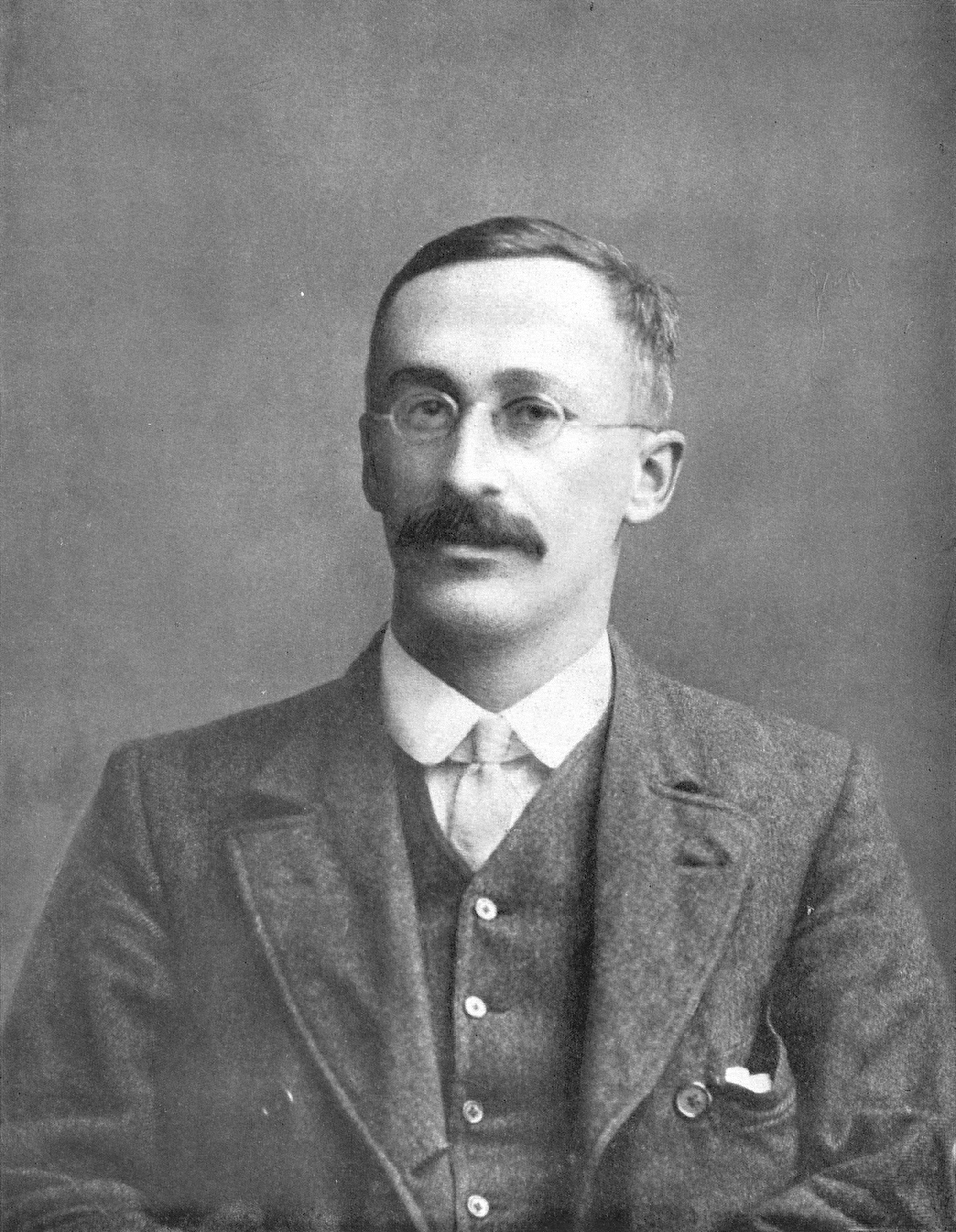
William Gossett and Student’s \(t\)

Harald Bischoff, CC BY-SA 3.0
link, via Wikimedia Commons

User Wujaszek on pl.wikipedia,
Public domain, via Wikimedia Commons
Calculate \(\bar{x}\) and \(S\).
Calculate \(S_{\bar{x}}\).
Choose a confidence level,
for example, \(95\%\) or \(p = 0.05\).
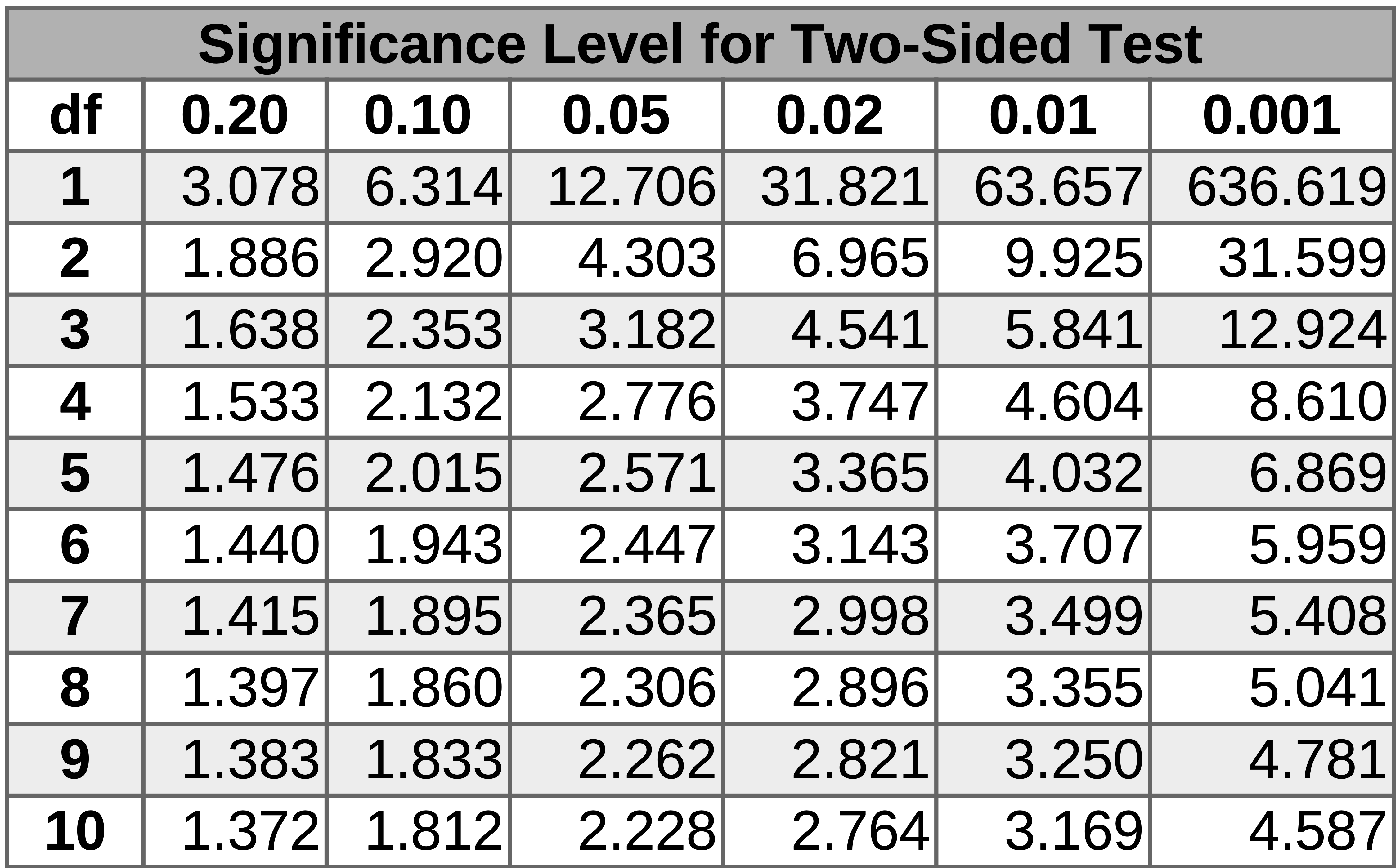
Find \(t\) given \(p\) and \(df = N - 1\).
Then \(\lambda = tS_{\bar{x}}\)
and \(\mu = \bar{x} \pm \lambda(1- p\ \mathrm{ conf.})\)
For example, \(x = 42.000 \pm 0.067(95\%\ \mathrm{conf.})\)
So \(\lambda\) is 1/2 the width of the confidence interval and the confidence interval width is \(2\lambda\).
Student’s \(t\) Table

For example, \(\bar{x}\) is \(42.000 \pm 0.067\) with 95% confidence.
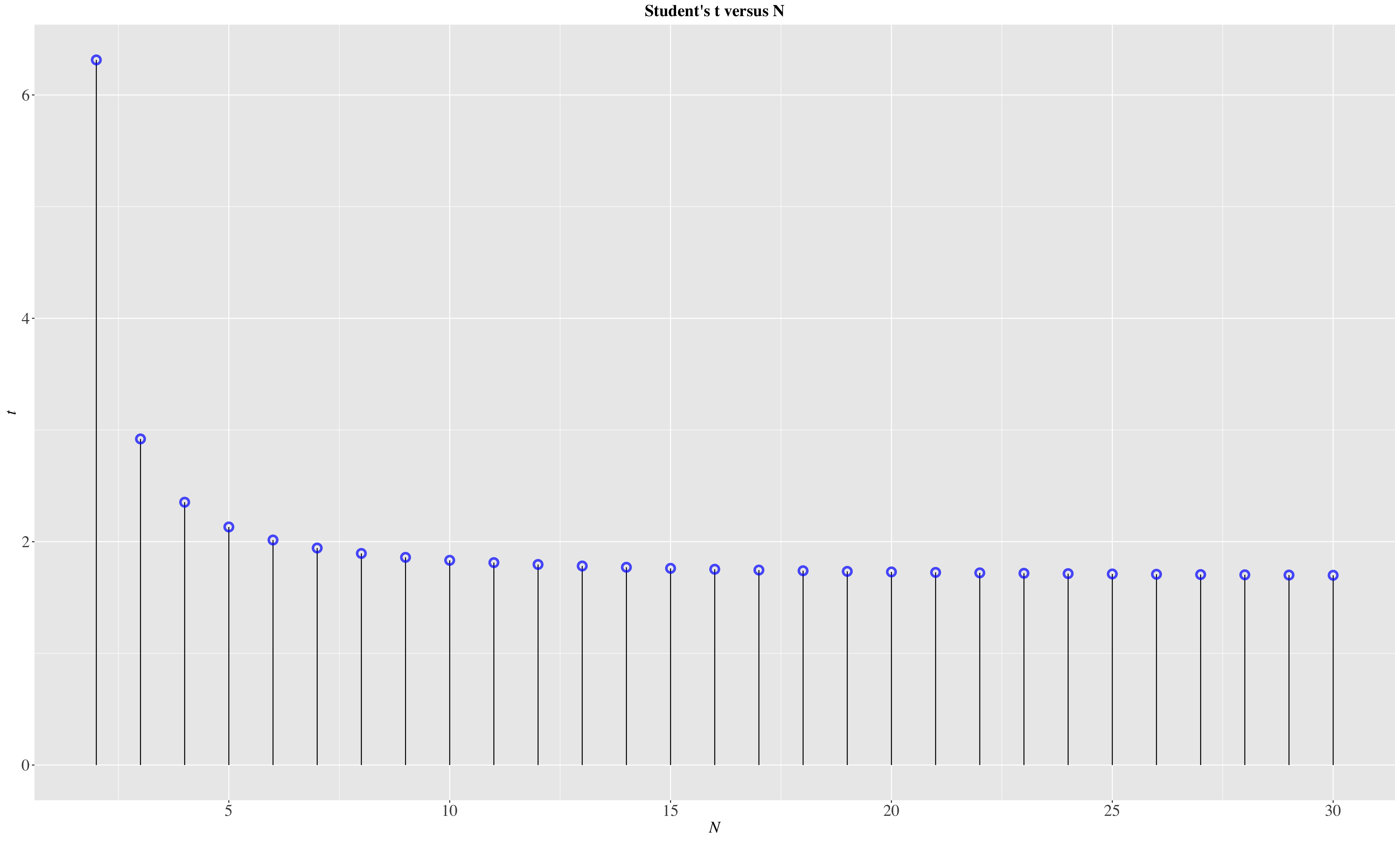
Effect of \(N\) on \(t\)
\(\lambda = tS_{\bar{x}}=\frac{tS}{\sqrt{N}}\)

Student’s \(t\) as a Function of \(N\)
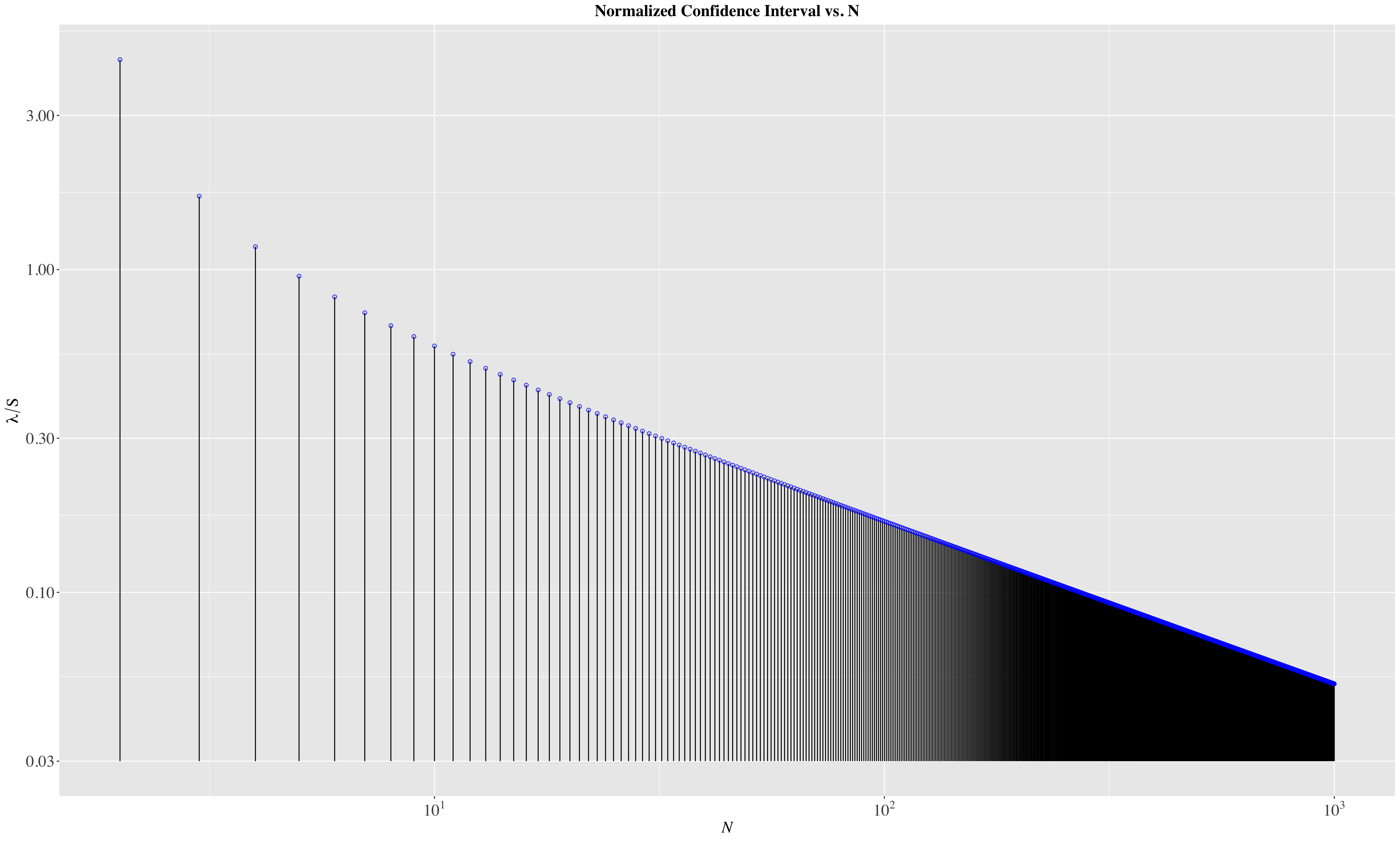
Effect of \(N\) on \(\lambda/S\)
\(\lambda = tS_{\bar{x}}=\frac{tS}{\sqrt{N}}\)

Normalized Conf. Int., \(\lambda/S\) as a Function of \(N\)
\(\mu,\ \bar{x},\ S\ ,\lambda\) Demo with Histogram
\(\ \ \ \)
\(\ \ \ \)
The Takeaways
- When measuring something, make at least three measurements, which gives you the greatest decrease in uncertainty per additional measurement.
- Use the methods in this video to calculate your confidence interval from the estimated standard error and the Student’s \(t\) value.
- Report your results with the mean of your measurements, the confidence interval and the confidence level: for example 42.000 plus-or-minus 0.067 at a 95% confidence level.
There are four additional videos showing how to perform these calculations by hand, with a spreadsheet, using Python and NumPy/SciPy, and using R.
Thanks for watching!
The Full Story companion video is in the link in the upper left. The first of the How To videos is in the upper right. To learn more about Chemical and Thermal Processes, visit the website linked in the description to find previous and following videos in this series.
The DOFPro Team

